21 Distributed serving and KV locality
Adding serving workers can increase the number of requests processed at once, yet moving an active request can delay its next token if its cache remains on another worker. Splitting one model across GPUs can solve a capacity limit, but it can also add communication inside every layer or decode step. The design must separate routing among complete serving groups from the work needed to execute a sharded model within a group.
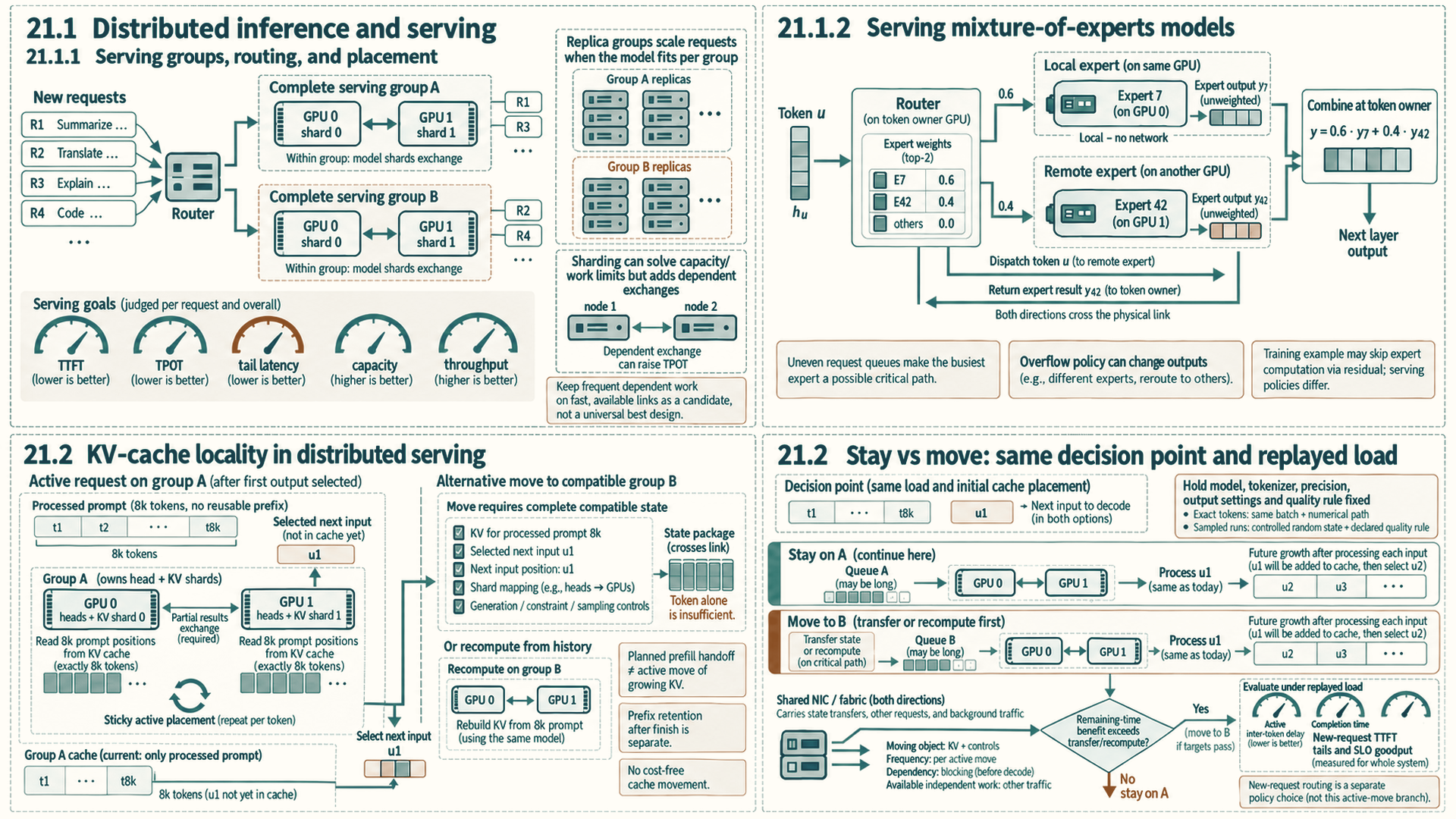
Three decisions meet at each request: how the model is placed, which group runs the request, and where that request’s key-value cache stays. A replica group can keep token generation local when the model fits. A sharded group must include its required exchanges in the latency and throughput measurements. Cache migration or recomputation is a further cost, so moving a request toward a less busy group helps only when the expected benefit outweighs that cost.
21.1 Distributed inference and serving
Distributed inference uses the same links, backends, and collective libraries as distributed training, while the user-facing metric changes. The goal includes latency, Time To First Token (TTFT), Time Per Output Token (TPOT), tail behavior, serving capacity, and tokens per second.
21.1.1 Serving groups, routing, and placement
A distributed serving system combines request routing and cache ownership with replica, tensor-parallel, or pipeline-parallel worker groups. vLLM and SGLang can coordinate multi-GPU serving groups. The TensorRT-LLM documentation retrieved September 28, 2026 describes PyTorch-native execution for supported models and multi-GPU configurations. Older releases used a compiled-engine workflow (Section 15.2.2). The software choice follows the placement strategy and topology rather than defining them.
The critical ownership questions are which worker group holds the model shard, which group owns each request’s KV cache, which collectives lie on every decode step, and whether routing preserves that locality across replicas.
A common serving strategy keeps frequent collectives inside a node and scales across nodes by replicating serving groups. This avoids making every token depend on a slow cross-node path. When the model is too large for one node, the system must balance model sharding, cache locality, batch scheduling, and network cost.
When a model fits inside a serving group, replicas can scale throughput without putting cross-node communication on every token. Larger models may need tensor or pipeline sharding, which adds collectives or activation transfers. Keep active requests near their KV state and measure token and tail latency.
- Tensor-parallel serving: Splits layer math across GPUs. It helps when one layer is too large or too slow for one GPU, but it may put collectives in the per-layer or per-token path, so fast intra-node links matter.
- Pipeline-parallel serving: Assigns different layer ranges to different devices. It can fit deeper models, but stage imbalance, micro-batch scheduling, and activation transfer can increase tail latency.
- Replica groups: A router sends requests to one of several complete serving instances. This is often simpler than cross-node sharding when the model fits per group, and it can preserve low Time Per Output Token (TPOT).
- Router and cache locality: The router should avoid moving an active request away from the devices holding its KV cache unless the benefit outweighs the transfer cost.
- Cross-node sharding: A capacity or throughput option when one node is insufficient or another placement goal justifies it. It carries higher decode-latency risk when each token depends on cross-node communication with little independent work to hide the cost.
Distributed inference can be slower than single-node inference when the model already fits and per-token communication dominates. A single optimized replica may produce lower TPOT than a cross-node sharded model because decode has little independent work to hide network latency. The correct scale-out design depends on whether the bottleneck is memory capacity, throughput, Time To First Token (TTFT), TPOT, or tail latency.
| Dimension | Training tensor parallelism | Inference tensor parallelism |
|---|---|---|
| Primary metric | Step throughput and model flops utilization | TTFT, TPOT, tail latency, goodput meeting the SLO |
| Batch shape | Large micro-batches can reduce collective time as a share of useful computation | Decode may have one token per sequence, so per-layer collectives are more exposed |
| Overlap opportunity | Layer collectives overlap only independent work; dependent forward outputs and backward input gradients must wait. DDP buckets belong to a separate data-parallel group | The next token or layer often needs the collective result immediately |
| State pressure | Activations, gradients, optimizer state, and parameters | Weights plus KV-cache placement and per-request cache locality |
| Topology rule | Cross-node TP needs enough compute per exchange or sufficiently fast links to keep exposed communication acceptable; overlap helps where dependencies permit it | Per-token TP should usually stay inside the fastest scale-up domain |
21.1.2 Serving mixture-of-experts models
A mixture-of-experts model separates the parameters it stores from the parameters each token uses. DeepSeek-V2, for example, has 236 billion parameters in total, of which 21 billion are activated for each token.1 A deployment must make all required expert weights available, while each token uses only its selected experts and shared components. Assuming all weights remain on GPUs in BF16, their payload is 472 GB, a capacity-only lower bound of six 80 GB GPUs before KV cache, workspaces, replication, or placement constraints. The coarse \(2P\) estimate gives about \(2\times21\times10^9=42\) GFLOP per token for parameter-related forward work, compared with 472 GFLOP when all 236B parameters are active (Section 2.2). This excludes attention’s context-dependent work and routing overhead. The active count alone therefore cannot predict memory needs or the serving bottleneck.
Expert parallelism places experts across GPUs, so remote token routes may require dispatch and combine transfers. Total weights differ from weights active per token. Few tokens per expert can give poor reuse, and a busy expert can set latency. If an expert's token buffer overflows, the engine may skip that expert's computation and change the output. Check the engine's policy.
- Expert parallelism in serving: Experts are spread across GPUs. In the dispatch/combine layout of Section 20.2, a layer routes token representations to remote experts and returns their outputs through two logical exchanges. An engine may implement these with all-to-all collectives or another schedule, and local routes need no cross-GPU transfer. Frequent remote routing favors a fast scale-up domain when capacity permits (Section 17.4).
- Tokens per expert: A step with \(B\) tokens and top-\(k\) routing over \(E\) experts has an average of \(Bk/E\) token assignments per expert before capacity limits. With 64 experts, top-2 routing, and 256 tokens, that average is 8 rows. Actual counts depend on the router. Eight-row multiplications often have little weight reuse and can be memory-bound (Section 6.2); dtype, matrix dimensions, caching, and grouped kernels affect the measured limit. Larger decode batches can raise rows per expert and arithmetic intensity when routing remains balanced.
- Load imbalance: The busiest expert or rank can set the expert phase’s completion time when its work lies on the critical path. For its top-1 routing, Switch Transformer sizes each expert’s buffer as the tokens per batch divided by the number of experts, times a capacity factor, and passes tokens that exceed it to the next layer through the residual connection without expert computation.2 Top-\(k\) engines may use different capacity accounting. Dropping an expert computation can change the model’s output, so a serving deployment checks how its engine handles overflow.
21.2 KV-cache locality in distributed serving
KV-cache locality is the serving-design property that keeps an active request near the GPU group holding its key-value cache blocks. It matters because decode repeatedly reads old KV blocks and appends new ones. Moving an active request away from its cache can add a large transfer or force recomputation.
A planned prefill/decode handoff sends initial KV and compatible request state to a decode worker before token generation continues there. Moving an already decoding request is a separate decision: its KV has grown with each emitted token, and the new group needs the compatible state required for the next step. The example below tests that active move.
The common pattern is Sticky placement: once a request has built substantial KV state on a serving group, the router prefers keeping later decode steps on that group unless the load-balancing benefit outweighs transfer or recomputation cost. This is a serving-scheduler property, not an attention-kernel or hardware-cache optimization.
- Sticky placement: An active request remains on the worker group that owns its current KV blocks.
- Locality-aware routing: New-request routing considers both load and whether useful prefix or cache state already exists on a worker.
- Cache migration: Moving KV blocks between worker groups. For load balancing, the expected benefit should outweigh peer, host, or network transfer cost. Prefill/decode handoff or worker evacuation can require movement for other reasons.
Example: One request on a sharded serving group
Setup: Groups A and B are separate serving groups. Each group has two GPUs holding one tensor-parallel copy of the same model, with attention heads and their KV state split across its GPUs. The groups use the same GPU type, model weights, precision, and execution configuration. Assume there is no reusable prefix. A CPU front end tokenizes an 8k-token prompt, and the router assigns this request to A. These are illustrative conditions, not benchmark results.
Prefill and first token: A’s scheduler admits the prompt under its token and cache budgets. Each GPU runs its assigned attention and projection work and stores KV blocks for its local heads. The GPUs combine partial layer outputs where the layout requires it; Section 19.1 traces one such tensor-parallel all-reduce. After prefill produces next-token scores, the sampler selects the first output token and the server emits it. The exact exchanges depend on the model and implementation.
Repeated decode and cache ownership: Both GPUs receive the selected token for the next step. Each reads and extends its own KV shard, performs its assigned layer work, and joins the required exchanges before the next token is selected. Decode repeats on A until the request stops. A then releases the request’s active cache ownership. Its separate prefix-cache policy may retain valid blocks for a future request; that reuse is not migration of this active request.
After A emits its first selected token, its KV cache still covers the processed prompt, as in the decode state trace. To continue on B, each B worker needs those KV blocks mapped to its corresponding layer and head shard, the next sequence position, and the selected token as its next input. B then processes that token, extends KV and selects the following token. For a later move, transfer KV for all already processed positions plus any selected token not yet processed. Recomputing from the token history can reconstruct the required KV state instead. The request’s generation limits, output constraints and sampling state, including random state when the chosen output rule needs it, must move with the request. Compatible weights and cache layout alone do not supply that control state.
Routing decision and fair check: Suppose B becomes less busy after the first token. Moving the active request to B requires transferring A’s KV state in a compatible layout or recomputing it on B. Sending only the latest token is insufficient. Compare keeping this request on A with moving it at the same decision point under a replay of the same arrivals and initial cache placement. Hold the model, tokenizer, precision, generation settings, and output-quality rule fixed.
For an exact-token comparison, hold batch composition and the numerical execution path fixed as well as using deterministic decoding, then verify outputs; a nearly tied greedy choice can change when batching or reduction order changes. If those conditions cannot be held, use the declared numerical or output-quality rule instead. For sampled runs, control random state and apply the declared quality rule rather than assuming individual outputs match. Include transfer and recomputation time.
Record the active request’s inter-token delay and completion time, new requests’ TTFT, transferred bytes, recomputed tokens, tail latency, and SLO goodput using the Section 15.1 request-load method. Routing new requests to B is a separate policy comparison.
Conclusion: B’s shorter queue helps only if its expected remaining-time benefit exceeds cache movement or recomputation and meets the latency and quality targets. Measure the whole sharded request path, including its internal exchanges.
The following table applies the communication frequencies introduced with topology-aware design to complete placement and scheduling patterns. Each row states the intended topology fit and the failure that appears when the mapping is wrong.
| Design pattern | Communication pattern | Topology fit | Failure mode |
|---|---|---|---|
| Topology-aware placement | Ranks with frequent exchange are placed near each other | Prefer NVLink/NVSwitch for frequent collectives; same-rack placement only helps when the measured network path meets the workload’s latency target | Scheduler spreads hot ranks across slow paths |
| Hierarchical collective | Communicate inside one scale-up domain, then across slower domains, then inside the destination scale-up domain | Matches intra-node GPU fabric plus cross-node network | Treats all rank pairs as equally cheap |
| Bucket and overlap | Group tensors and launch communication while compute continues | Works when independent compute remains | Small buckets add overhead; large buckets expose a tail |
| Shard-and-gather | Store state sharded; materialize only near layer use | Works when gather/reduce paths are fast enough | Memory saved locally becomes network-bound |
| Scale-up first, scale-out second | Keep per-token or per-layer traffic inside one node/group | Serving replicas or groups scale across nodes | Exposed cross-node per-token exchanges can raise TPOT when their delay exceeds saved compute |
| Sticky KV-cache placement | Route active requests near the GPUs holding their KV cache | Serving groups with stable cache locality | Load balancing moves cache-heavy requests too freely |
| Rail or NIC-aware grouping | Ranks that leave a node use the intended NIC path | Systems with multiple NICs or network rails | Traffic concentrates on one weak interface |
| Topology-aware replica placement | Replicas are spread to avoid shared-fabric hot spots | Serving fleets and multi-tenant clusters | All replicas contend on the same leaf or spine |
Design checklist
Object: Is the moving object a gradient, parameter shard, activation, KV block, expert token, logits vector, request, or checkpoint chunk?
Frequency: Does it move per token, per layer, per step, per request, or in the background?
Critical path: Would shortening this transfer reduce TTFT, TPOT, step time, or tail latency?
Overlap: Is there independent compute available while the transfer runs?
Locality: Does the traffic stay inside the intended scale-up domain, or does it cross NICs and switches?
Contention: What happens when multiple jobs, collectives, or serving replicas share the same fabric?
Metric: Is success judged by throughput, TTFT, TPOT, tail latency, utilization, memory capacity, or cost?
Comparing these patterns helps expose a common distributed-system error: choosing a parallelism strategy because it fits memory, then discovering that its communication frequency does not fit the topology. Memory capacity and communication distance have to be designed together.
The measured hot path determines the placement. Replicated groups can scale request throughput without adding per-token cross-node collectives when the model fits per group. A sharded group can solve capacity or parallel-compute limits, but its per-layer or per-token communication must be included in TTFT, TPOT, throughput, and tail-latency measurements.
Appendix A collects the formulas, software controls, compatibility checks, practice questions, and source map needed to apply the same reasoning during implementation and review.
References
DeepSeek-AI. (2024). DeepSeek-V2: A Strong, Economical, and Efficient Mixture-of-Experts Language Model. arXiv:2405.04434. Supports 236B total parameters with 21B activated per token. Limit: the memory and FLOP figures in the distributed serving estimate are derived from these counts.↩︎
Fedus, W., Zoph, B., & Shazeer, N. (2022). Switch Transformers: Scaling to Trillion Parameter Models with Simple and Efficient Sparsity. Journal of Machine Learning Research, 23(120), 1-39. Journal article; arXiv:2101.03961. Supports expert capacity = (tokens per batch / number of experts) x capacity factor, and dropped tokens passing to the next layer through the residual connection. Limit: the paper describes training, and inference engines handle overflow in their own ways.↩︎