6 Performance models
A roofline model combines the arithmetic work and memory traffic of a defined region with compute and bandwidth ceilings. The counts depend on the operation and phase: training backward, prompt prefill and one-token decode can move different data even with the same model weights.
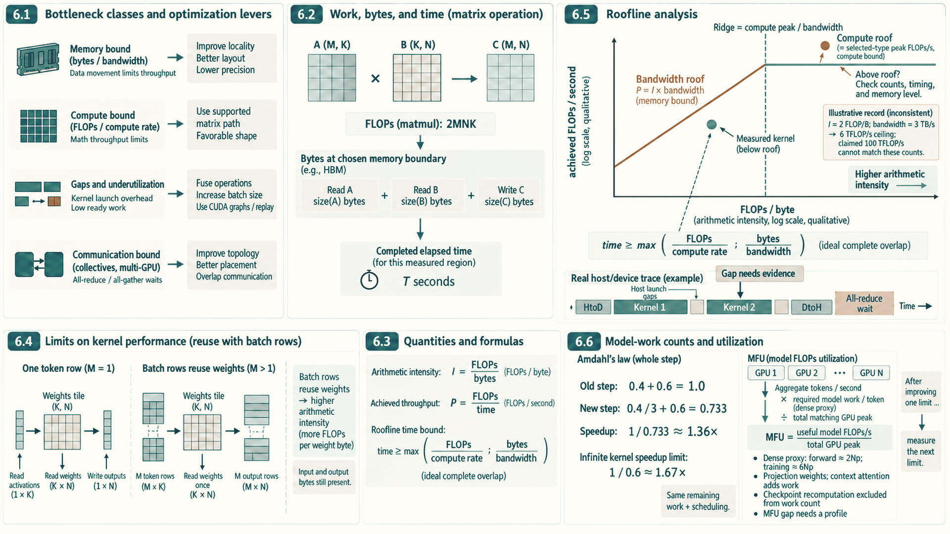
Elapsed time places a measured result against those ceilings. A point below the roof shows a gap to the ideal bound; it does not identify the cause or prove that the gap can be closed. Launch overhead, synchronization, communication, cache behavior and inaccurate counts can all affect the comparison. Profiler selection in Section 7.2.1 explains the evidence used to distinguish them.
A bottleneck is the resource or dependency that currently limits one measured execution region. It is not a permanent label for the whole model: a training forward pass, an optimizer update, prompt prefill, one-token decode, and distributed synchronization can each be limited by a different resource.
6.1 Bottleneck classes and optimization levers
A measurement names the slow region. The next decision is what kind of limit that region hits, because each kind has its own family of fixes. Two classifications organize the rest of the guide: bottleneck classes describe what limits a region, and optimization levers describe what a change does.
A region’s bottleneck class identifies its limiting resource or wait. Capacity can instead limit whether the requested work fits at all. Tensor storage (Section 1.2) tells us how many bytes each object occupies. Live state and memory (Section 2.1) explains which objects stay live together and set peak memory. Workload phases (Section 2.2) and the training step (Section 2.3) identify which computation, transfers, and waits belong to the region being timed. These connections determine the measurements: arithmetic, bytes transferred, peak storage, and time spent waiting. Each class describes one region under measured conditions, not a permanent property of the model.
When a region runs near its arithmetic throughput limit, it is compute-bound. When transfers run near the bandwidth limit of a memory tier, it is memory-bound. A latency-bound region has too little parallel work to hide memory or instruction delays, so neither throughput limit is reached. NVIDIA GPUs schedule threads in groups of 32. Each group is a warp. Occupancy, the fraction of supported warps active on a GPU processing unit, is one clue to available parallel work (Section 3.1); it is not a speed measurement by itself.
A lever applied to one region improves the whole run only in proportion to that region’s share of the time. If a non-overlapped fraction \(f\) of the step time is sped up by a factor \(k\) and the remaining work and scheduling are unchanged, the new step takes \((1-f)+f/k\) of the old time, so the overall speedup is
\[ \text{speedup}=\frac{1}{(1-f)+f/k}. \]
This relation is Amdahl’s law.1
Example: A 3x faster kernel
Inputs: One kernel takes 40 percent of a training step (\(f=0.4\)), and a rewrite makes it three times faster (\(k=3\)).
Calculation: The new step takes \(0.6+0.4/3\approx0.733\) of the old time, a speedup of \(1/0.733\approx1.36\times\). Even an infinitely fast kernel gives at most \(1/0.6\approx1.67\times\).
Conclusion: A region’s share of the time bounds what any lever applied to it can achieve, so measuring the share comes before choosing the fix. After the change, a new measurement identifies the resource or wait limiting the remaining exposed work. The largest remaining time share is a useful place to investigate, but its cause still needs evidence. The limiting region can move as described in Section 2.2.
6.2 Work, bytes, and time
For a first projection-only estimate, one multiplication and one addition per weight give \(2N_p\) floating-point operations (FLOPs) per token. Taking \(N_p=8\times10^9\) gives 16 GFLOP, roughly 16 microseconds at an H100’s dense BF16 peak. The model-work estimate below states the omitted operations and attention term. For a model whose projection weights exceed cache capacity, a small decode step typically reads most of those weights from HBM, so memory traffic can set the time. Arithmetic and data movement each impose a lower bound. Their maximum is an ideal estimate when they overlap completely. Choosing the right optimization therefore starts with knowing which of the two is slower.
To a first approximation, arithmetic takes FLOPs divided by the peak compute rate, and data movement takes bytes moved divided by the memory bandwidth. Their ratio depends on one property of the operation:
- Arithmetic intensity: FLOPs performed per byte moved to or from memory, measured in FLOP/byte. It states how much arithmetic each fetched byte supports.
- Ridge point: the peak compute rate divided by the memory bandwidth. At this intensity the two times are equal.
- Memory-bound and compute-bound regions: below the ridge point, the bandwidth ceiling is lower than the compute ceiling. Above it, the compute ceiling is lower. These are the model’s limiting resources. A measured kernel can still be limited by launch overhead, latency, or poor utilization.
For an H100 SXM GPU, the dense BF16 Tensor Core peak is about 989 TFLOP/s. NVIDIA’s specification lists 1,979 TFLOP/s with structured sparsity, twice the dense rate. With 3.35 TB/s of HBM bandwidth, the ridge point is \(989\times10^{12}/3.35\times10^{12}\approx295\) FLOP/byte.2 A BF16 operation must therefore perform about 295 arithmetic operations for every byte it moves before the arithmetic units, rather than memory, become the limit.
Several token rows can reuse each loaded weight. Increasing the number of rows therefore adds arithmetic without requiring a separate weight read for each row, although input and output traffic also grows. This raises arithmetic intensity and can move the operation toward the compute limit.
Example: One projection at four batch sizes
Inputs: A BF16 weight matrix of shape \(4{,}096\times4{,}096\) multiplies a batch of \(B\) token vectors of width 4,096, the query projection from Section 1.1. Each weight is used once per row in one multiply and one add, so the operation performs \(2\times B\times4{,}096^2=33{,}554{,}432\,B\) FLOPs. It reads the weights once (\(2\times4{,}096^2=33{,}554{,}432\) bytes) and reads and writes \(B\) rows of 4,096 two-byte values (\(16{,}384\,B\) bytes). The intensity is therefore \(33{,}554{,}432\,B/(33{,}554{,}432+16{,}384\,B)=B/(1+B/2{,}048)\) FLOP/byte.
| Rows \(B\) | FLOPs | Bytes moved | Intensity (FLOP/byte) | Time at 3.35 TB/s | Time at 989 TFLOP/s | Limit |
|---|---|---|---|---|---|---|
| 1 | 33.6 M | 33.6 MB | 1.0 | 10.0 µs | 0.03 µs | Memory |
| 64 | 2.15 G | 34.6 MB | 62 | 10.3 µs | 2.2 µs | Memory |
| 345 | 11.6 G | 39.2 MB | 295 | 11.7 µs | 11.7 µs | Balanced |
| 2,048 | 68.7 G | 67.1 MB | 1,024 | 20.0 µs | 69.5 µs | Compute |
Conclusion: With one row, which is one token of single-request decode, each weight byte supports about one FLOP, nearly 300 times below the ridge point. Under this HBM-traffic estimate, the memory-time lower bound is about 10 microseconds. Adding rows reuses each loaded weight, so this ideal bound grows slowly until about 345 rows, where the compute and memory bounds meet. This is why prefill and training, which process many tokens at once, tend to be compute-bound, while small-batch decode tends to be memory-bound. The estimate assumes that the weights come from HBM and that copying and computing overlap perfectly.
These two times give a lower bound, not a prediction. A kernel can be slower than both because of launch overhead, too little parallel work, poor memory access patterns, or synchronization. The counting rules and roofline model below generalize this projection estimate. The following measurement chapter then compares the bound with completed GPU work. The earlier matrix-vector explanation shows how access and parallelism affect the gap; the later decode chapter applies the same work-and-byte reasoning to a complete generation step.
6.3 Quantities and formulas
Performance models compare measured work, elapsed time, and data movement. The core quantities are floating-point operations, bytes moved through the memory level being modeled, arithmetic intensity, and achieved throughput. Section 6.2 introduced arithmetic intensity and the ridge point. This section fixes the counting rules they depend on, because both the roofline model and profiler results use them. Arithmetic intensity is written as:
\[ \text{AI} = \frac{\text{FLOPs}}{\text{bytes moved}} \tag{6.1}\]
The numerator and denominator must describe the same measured region and memory boundary. The definitions below make those counting choices explicit.
- AI: Arithmetic intensity, measured in FLOPs per byte. Higher AI means more arithmetic is performed for each byte moved.
- FLOPs: Floating-point operations performed by the kernel or phase. The count must match the operation being timed.
- bytes moved: Estimated traffic through the memory level being modeled, usually HBM for a first roofline pass. If the byte estimate ignores cache reuse or temporary buffers, the roofline conclusion can be wrong.
For example, 2e12 FLOPs and 1e12 bytes gives AI = 2 FLOPs/byte. The formula is useful because it forces an explicit byte estimate, but it omits cache effects, compression, metadata traffic, and hidden workspace movement.
| Workload fragment | First byte-count estimate | What the estimate misses |
|---|---|---|
| Vector read and write | Read n elements and write n elements: about 2 x n x dtype_bytes | Cache reuse, write allocation policy, alignment, and vectorized transaction granularity. |
| GEMV y = Ax | Read M x N matrix values, read N vector values, and write M outputs | Repeated vector reuse from cache, partial sums in registers, batching, and fused final operations, such as bias or activation. |
| GEMM C = AB | Read A and B and write C as a lower bound | Tiling can reuse A and B many times from on-chip storage, while poor tiling can add extra movement. |
| Naive attention scores | Materializing scores costs batch x heads x sequence x sequence x dtype_bytes for the score tensor alone | Masks, softmax temporaries, dropout, and whether an IO-aware kernel avoids the score tensor entirely. |
| KV-cache decode read | Read cached K and V for active tokens, layers, KV heads, head dimension, and dtype | Paged-cache metadata, cache locality, sharing key/value heads among query heads, quantized cache formats, and batching policy. |
The arithmetic count can be derived from the same dimensions as the byte estimate. In C = AB, with shapes (M, K), (K, N), and (M, N), there are M*N output entries. Each accumulates K products. Counting one multiply plus one add as two FLOPs gives the usual estimate 2*M*N*K, even when a fused multiply-add is one machine instruction3. This convention starts each output accumulator at zero and counts K multiplications and K additions, including the first addition to zero. A dot product written as K multiplies and K-1 additions has an exact algebraic count of 2*K-1 instead. Bias, activation, output scaling, and other final operations are additional work if they are inside the measured region. For Chapter 5’s GEMV, A has shape (M, N), so the same convention gives 2*M*N FLOPs.
Achieved throughput is computed from the measured runtime:
\[ \text{achieved throughput} = \frac{\text{FLOPs}}{\text{seconds}} \tag{6.2}\]
This quotient is valid only when the operation count and elapsed time cover the same work. Reporting the operation count, elapsed time, and rate together makes the measurement checkable.
- FLOPs: The same operation count used in the roofline estimate.
- seconds: Measured elapsed time for the same region. Include launch, synchronization, and communication only if those costs are part of the question.
- throughput: Measured work rate, usually reported as TFLOP/s for deep learning kernels.
If the same 2e12-FLOP kernel runs in 0.020 seconds, achieved throughput is 100 TFLOP/s. This is an illustrative rate calculation, not a reported measurement or a hardware property. It becomes misleading when warmup, compilation, or unrelated synchronization is included accidentally.
Monitoring tools report a different quantity under a similar name. The “GPU utilization” shown by nvidia-smi is the percentage of time over the sample period during which one or more kernels was executing on the GPU.4 A single small kernel running continuously reports 100 percent while it occupies a tiny fraction of the SMs and arithmetic units. That figure therefore detects idle gaps between kernels, but it cannot show how efficiently the GPU works while kernels run. MFU and the kernel metrics in Section 7.2.2 can.
A roofline estimate compares the compute ceiling with the bandwidth ceiling5:
\[ \text{roofline bound} = \min(\text{peak compute}, \text{AI} \times \text{peak bandwidth}) \tag{6.3}\]
The ridge point is the arithmetic intensity where the bandwidth ceiling reaches the compute ceiling:
\[ \text{AI}_{\text{ridge}} = \frac{\text{peak compute}}{\text{peak memory bandwidth}} \tag{6.4}\]
The two ceilings must refer to the selected dtype, operation path, and memory tier. These terms determine which side of the ridge point the workload occupies.
- peak compute: Best plausible arithmetic throughput for the selected precision, GPU generation, and kernel path. FP16, BF16, TF32 (NVIDIA’s reduced-precision mode for FP32 matrix math, Section 9.4), FP8, and integer formats have different ceilings.
- peak bandwidth: Relevant memory bandwidth for the modeled path. HBM bandwidth is not the same as NVLink, PCIe, or network bandwidth.
- AI times peak bandwidth: The bandwidth ceiling expressed as FLOP/s. It says how much compute can be sustained if every byte must be supplied at that bandwidth.
- ridge point: Arithmetic intensity at which the bandwidth ceiling and compute ceiling meet. Left of the ridge, bandwidth is the first-order limit. Right of the ridge, compute throughput is the first-order limit.
If AI = 2 FLOPs/byte and bandwidth is 3 TB/s, the memory ceiling is 6 TFLOP/s, so a 200 TFLOP/s compute peak does not matter for that kernel until reuse improves. The roofline omits scheduler overhead, launch overhead, synchronization, imperfect occupancy, dynamic shapes, and distributed communication.
For an illustrative FP16 matrix product with M=64, N=32, and K=128, the one-read-per-input, one-write-per-output estimate gives about 18.29 FLOPs per byte. At matching ceilings of 200 TFLOP/s and 3 TB/s, bandwidth caps the roof at about 54.86 TFLOP/s. That ceiling is not achieved speed, especially for this small launch.
Example: From matrix dimensions to a roofline bound
Inputs and work: Consider C = AB with M=64, N=32, and K=128, FP16 inputs and output, and no bias or read of an old C. There are 64*32 = 2,048 output entries, each with 128 multiply-add steps. At two FLOPs per step, the count is 2*64*32*128 = 524,288 FLOPs.
Bytes and intensity: Using the table’s one-read-per-input, one-write-per-output estimate gives 2*(64*128 + 128*32 + 64*32) = 28,672 bytes. FP16 occupies two bytes per stored value regardless of a wider accumulator. Arithmetic intensity is 524,288 / 28,672, approximately 18.29 FLOPs/byte.
Ceiling and interpretation: For illustrative matching ceilings of 200 TFLOP/s and 3 TB/s, the bandwidth roof is 18.29*3 = 54.86 TFLOP/s, below the compute roof. The model therefore predicts a bandwidth ceiling of about 54.86 TFLOP/s, not an achieved speed. The tiny shape can also be limited by launch overhead. Repeated HBM reads or extra writes increase the byte count and lower this roof, while inputs already in cache require a different HBM traffic estimate. No measured runtime is supplied for this calculation.
6.4 Limits on kernel performance
A measured region can take longer because it is moving bytes, performing arithmetic, waiting on dispatch, or waiting for other devices. The following labels make those causes explicit.
These categories are diagnostic, not labels for whole applications. One training step can contain compute-bound GEMMs, memory-bound optimizer updates, launch-bound small operations, and communication-bound gradient synchronization. The right optimization depends on the region being measured.
The following four labels describe a measured region. Each names the dominant cost and points to the first change worth testing:
- Memory-bound: Runtime follows bytes moved. Key-value cache reads during decode are a common example. Test locality, precision, coalescing, and cache layout.
- Compute-bound: Runtime follows arithmetic throughput. Large dense projections are a common example. Test Tensor Core use, dimension alignment, and useful batch size.
- Launch-bound: GPU work is short and CPU or dispatch gaps dominate. Many small eager operations are a common example. Test fusion, compilation, or CUDA Graph replay.
- Communication-bound: Collectives dominate the timeline. Distributed gradient synchronization is a common example. Test overlap, sharding, rank placement, and topology.
These four classes connect the local work to possible limits. The following measurement chapter adds evidence for launch, input, communication and scheduler waits in trace interpretation. Arithmetic intensity then tests whether memory bandwidth or compute throughput can explain the measured region.
6.5 Roofline analysis
A roofline derivation turns a measured or estimated kernel into a ceiling comparison. The input is FLOPs, bytes moved, elapsed time, peak compute, and memory bandwidth. The output is a first-order explanation of whether the kernel is plausibly limited by memory traffic or arithmetic throughput.
Constructing the model: The roofline chart places achieved throughput against arithmetic intensity on a log-log scale. Its diagonal memory-bandwidth ceiling and horizontal compute ceiling meet at the ridge point, which separates the first-order bandwidth-limited and compute-limited regions.
For one measured region, FLOPs divided by bytes moved place the point on the horizontal axis, while FLOPs divided by elapsed time place it on the vertical axis. The comparison uses bandwidth and compute ceilings for the same dtype, operation path, and memory level.
In the first-order model, points left of the ridge are bounded by the memory roof and points right of it by the compute roof. A point below either roof still requires profiling before choosing a kernel, precision, or hardware change.
Low arithmetic intensity means the bandwidth ceiling is low. High arithmetic intensity can move the kernel toward the compute ceiling. The ridge point is the diagnostic boundary: to the left, reduce bytes or increase reuse. To the right, improve arithmetic throughput, tensor-core utilization, or useful batch shape.
The derivation is deliberately approximate. If the measured point appears above the roofline, the FLOP count, byte estimate, measurement window, or peak numbers are inconsistent. That inconsistency is useful because it forces the engineer to refine the model before choosing an optimization.
Roofline limit
Peak compute and peak HBM bandwidth define an upper bound. Real kernels can sit below it because of instruction mix, occupancy limits, shared-memory bank conflicts, register spilling, Tensor Core alignment, synchronization, launch overhead, cache misses, or incomplete overlap. Profiler evidence explains the gap below the bound.
A point below the roofline shows a gap to the ideal bound but does not identify whether launch gaps, occupancy, synchronization, or cache behavior caused it. The next question is whether a worked set of FLOPs, bytes, and elapsed time is internally consistent before an optimization is selected.
Worked roofline interpretation: A worked roofline pass counts FLOPs, estimates bytes moved, and measures runtime, then forms the two quantities below. The calculation that follows checks whether they are consistent with the hardware ceilings.
\[ \text{AI} = \frac{2 \times 10^{12} \text{ FLOPs}}{10^{12} \text{ bytes}} = 2 \text{ FLOPs/byte} \tag{6.5}\]
\[ \text{achieved throughput} = \frac{2 \times 10^{12} \text{ FLOPs}}{0.020 \text{ s}} = 100 \text{ TFLOP/s} \tag{6.6}\]
Example: Roofline diagnosis
Illustrative measurement record: Suppose the same region as in Section 6.3 has 2e12 FLOPs counted, 1e12 bytes estimated for that region, and 0.020 seconds recorded. The target GPU has a 3 TB/s peak-bandwidth estimate.
Arithmetic intensity: 2e12 / 1e12 = 2 FLOPs per byte.
Achieved throughput: 2e12 / 0.020 s = 100 TFLOP/s.
First-order ceiling: 2 FLOPs/byte x 3 TB/s = 6 TFLOP/s. The measured 100 TFLOP/s is above that ceiling, so the byte estimate, FLOP count, timing region, or assumed memory level must be wrong.
Next measurement: Profiler bytes, cache reuse, operation count, and timing boundaries identify the assumption that needs refinement before a kernel change is selected.
In LLM inference, this is why prefill and decode should not be tuned with one mental model. Large prefill projections are GEMM-like and can move toward the compute side of the roofline. Small-batch decode is often GEMV-like, repeatedly reading weights and key-value cache for few new tokens, so it tends to remain left of the ridge and bandwidth-sensitive unless batching or fusion changes the shape.
6.6 Model-work counts and utilization
A first estimate of dense projection arithmetic uses the number \(N_p\) of weights participating in those projections. Each such weight contributes one multiplication and one addition per token, giving about \(2N_p\) FLOPs per token. Backward propagation costs about twice the forward pass, so training costs about \(6N_p\) FLOPs per token.6 This estimate omits embedding lookup, normalization, and other smaller operations; an embedding lookup does not multiply every entry in its table. The cited scaling-law estimate excludes embedding parameters. Attention adds a term that grows with context length. That term is small when the context is short relative to the hidden width.
Example: Arithmetic per token for an 8B model
Inputs: Use \(N_p=8\times10^9\) as a rough proxy for the dense projection parameter count at the Llama 3 8B scale from Section 1.1, with the attention term ignored. This rounded estimate is not an exact operation count for that model’s embedding and output layers.
Inference: One forward pass per generated token costs \(2\times8\times10^9=1.6\times10^{10}\) FLOPs, or 16 GFLOP.
Training: One training token costs \(6\times8\times10^9=4.8\times10^{10}\) FLOPs. Training on \(10^{12}\) tokens therefore costs \(4.8\times10^{22}\) FLOPs. One H100 SXM running at its dense BF16 peak of about \(989\) TFLOP/s (Section 6.2) would need \(4.8\times10^{22}/9.89\times10^{14}\approx4.9\times10^{7}\) seconds, about 560 days, and real runs achieve only a fraction of peak.
Conclusion: The rough training work scales with participating projection weights times tokens, which helps explain the use of many GPUs (Chapter 18 and Chapter 19). For one generated token, 16 GFLOP would take about 16 microseconds at the stated peak rate. If each token step must read the model’s 16 GB of BF16 weights from HBM, that read alone takes at least about 4.8 milliseconds at 3.35 TB/s, roughly 300 times the arithmetic lower bound. This comparison shows why weight traffic can dominate a small, poorly reused decode step under those assumptions; cache reuse, batching, launch costs, and the actual kernel path determine measured time (Section 6.2).
Moving bottlenecks are normal. Removing recomputation can expose memory bandwidth. Increasing batch size can expose KV-cache capacity. Sharding model state can expose network synchronization. The engineering task is to follow the bottleneck as each change exposes a new constraint.
Achieved FLOP/s describes one kernel. A training run needs the same question answered for the whole model. Model FLOPs utilization (MFU) is the ratio of the arithmetic rate the model requires to the hardware’s peak rate: tokens processed per second times FLOPs per token, divided by the peak FLOP/s of the GPUs. For training, a rough dense-model estimate is \(6N_p\) FLOPs per token, using the projection-weight counting convention, plus an attention term that grows with sequence length. MFU counts only the operations that forward and backward passes require, so activation-checkpointing recomputation is excluded from its operation count. Checkpointing can still change MFU by changing achieved tokens per second. Comparisons need the same model-work convention and matching dtype-specific hardware peaks.7
Example: MFU of a training run
Inputs: An 8B-parameter model trains across eight H100 SXM GPUs at an illustrative aggregate 64,000 tokens per second. Each GPU’s dense BF16 peak is about 989 TFLOP/s (Section 6.2). The 8B parameter count is used as the same rough projection-count proxy, and the attention term is ignored. This is an arithmetic example, not a measured run. The model and training state must be distributed with a per-GPU memory budget as described in Chapter 18 and Chapter 19.
Calculation: The model requires \(64{,}000\times6\times8\times10^9=3.072\times10^{15}\) FLOP/s. Dividing by the eight GPUs’ total peak, \(8\times9.89\times10^{14}=7.912\times10^{15}\) FLOP/s gives an MFU of about 39 percent.
Conclusion: MFU compares runs by the useful arithmetic they complete. The gap to peak does not identify a time breakdown. Memory-bound work, recomputation, communication, launch gaps, instruction mix, and idle time can all contribute. A profile is needed to distinguish them.
References
Amdahl, G. M. (1967). Validity of the single processor approach to achieving large scale computing capabilities. In Proceedings of the April 18-20, 1967, Spring Joint Computer Conference (AFIPS ’67 Spring), 483-485. Amdahl’s paper at ACM. Source of the argument that the serial fraction of a workload limits overall speedup. Limit: the formula in Section 6.1 is the standard modern statement of that argument, not a quotation from the paper.↩︎
NVIDIA. (n.d.). NVIDIA H100 Tensor Core GPU product specifications. NVIDIA H100 performance specifications. Support: the H100 SXM column lists BFLOAT16 Tensor Core performance of 1,979 teraFLOPS, footnoted “With sparsity,” and 3.35 TB/s GPU memory bandwidth. Limit: the dense value of about 989 TFLOP/s is half the listed sparse figure, and both are theoretical peaks that depend on clocks and kernel path.↩︎
NVIDIA. (2023). Matrix Multiplication Background User’s Guide, section 2, Math and Memory Bounds (last updated 2023-02-01). Matrix Multiplication Background User Guide. Supports the two-FLOP multiply-add convention and 2MN*K GEMM estimate. Limit: arithmetic counts omit output scaling and other final operations unless added explicitly. The chapter’s small-shape calculation and hardware ceilings are illustrative. This source is also used in Chapter 3.↩︎
NVIDIA. (n.d.). nvidia-smi documentation.
nvidia-smidocumentation. Support: the Utilization GPU field is the percentage of time over the past sample period during which one or more kernels was executing on the GPU. The sample period ranges from 1 second to 1/6 second depending on the product. Limit: the field does not measure how much of each SM or arithmetic unit is in use.↩︎Williams, S., Waterman, A., & Patterson, D. (2009). Roofline: An Insightful Visual Performance Model for Multicore Architectures. Communications of the ACM, 52(4), 65-76. Roofline paper (DOI). Supports the ceiling form min(peak compute, operational intensity times peak bandwidth), the ridge point where the roofs meet, and the bound and bottleneck reading used in Sections 6.3 and 6.5. Limit: the paper models DRAM traffic after cache filtering on multicore CPUs; the chapter applies the same first-order reading to GPU HBM as a teaching model and adds GPU specific gaps separately.↩︎
Kaplan, J., et al. (2020). Scaling Laws for Neural Language Models. arXiv:2001.08361. Section 2.1 and Table 1 estimate forward compute as about 2N plus a context-dependent attention term per token, and training compute as about 6N FLOPs per token after accounting for the backward pass. Limit: N excludes embedding parameters, and the attention term matters when context length is large relative to model width.↩︎
Chowdhery, A., et al. (2022). PaLM: Scaling Language Modeling with Pathways. arXiv:2204.02311. Section 4.1 defines model FLOPs utilization as observed tokens per second relative to the theoretical maximum at peak FLOPs, counting only the forward and backward operations and not rematerialization. Appendix B gives 6N matmul FLOPs per token plus 6LH(2QT) for dense attention. Limit: the chapter’s aggregate 64,000 tokens/s on eight GPUs is an illustrative input, not a reported result.↩︎