16 Collective data movement and its cost
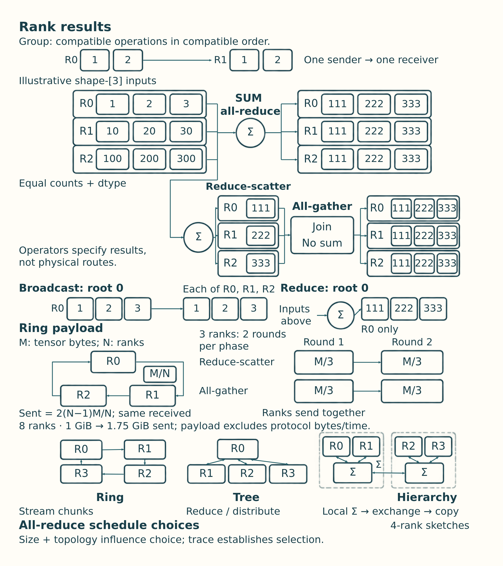
When several ranks hold pieces of one result, first ask what value each rank must receive. An all-reduce gives every rank the reduction of all inputs. A Reduce-scatter combines those inputs but leaves each rank with only part of the result. An All-gather collects held parts so every rank receives the whole array. These are result rules; a ring, tree, or network route is a later choice about how to produce them.
16.1 Point-to-point and collective communication
Distributed programs communicate either through explicit pairwise transfers or through group operations. The choice changes both the code structure and the synchronization behavior.
- Point-to-point communication: One rank sends data to another rank. It is common in pipeline stages, custom protocols, explicit activation transfers, and control paths where the communication pattern is irregular.
- Collective communication: A group of ranks participates in one operation with a defined group-level result, such as all-reduce, all-gather, or all-to-all.
- Ordering requirement: Ranks must call compatible collectives in compatible order. Mismatched ordering can hang or corrupt the distributed program.
- Point-to-point versus collective trade-off: Point-to-point communication can be flexible but harder to reason about globally. Collectives are structured and optimized, but they create synchronization points.
The semantics define who participates and which ranks receive results. They do not prescribe a central coordinator or physical traffic path.
16.2 Collective primitives
A collective operation is a group communication primitive used by strategies such as Distributed Data Parallel (DDP) for gradient synchronization, Fully Sharded Data Parallel (FSDP) for sharded model state, tensor parallelism for layer-internal slices, and expert parallelism for routed token state.
- Broadcast: One source rank sends the same tensor to every other rank. It copies a source value and is commonly used to initialize or synchronize parameters.
- Reduce: Many ranks contribute tensors that are combined on one destination rank. Use Reduce when only one rank needs the combined result. Use all-reduce when every rank needs it.
- All-reduce: All ranks contribute tensors, the tensors are reduced, and every rank receives the reduced result. DDP uses it for gradient synchronization and pays both reduction and redistribution traffic.
- All-gather: Each rank starts with a shard, and all ranks receive the full collection of shards. Materializing sharded parameters or activations creates a full temporary result on every participant.
- Reduce-scatter: Ranks reduce tensors and each rank receives one shard of the reduced result. FSDP and sharded optimizer paths use its combined reduction and partitioning behavior.
- All-to-all: Every rank sends a different slice to every other rank and receives different slices back. Expert-parallel token routing uses this latency-sensitive and topology-sensitive exchange.
The following array trace uses NCCL’s equal-count collective contracts and rank-ordered layouts.1 This example has equal counts and one dtype on all ranks. Uneven routing needs padding or an interface with explicit split sizes rather than assuming this contract covers it.
Example: Reduction, collection, and slice exchange
Three ranks use float32 arrays, compatible calls in the same order, and SUM where a reduction is required. Each six-element input has three consecutive two-element chunks, numbered 0, 1, and 2:
| Rank | Input, shape [6] |
|---|---|
| 0 | [1, 2, 3, 4, 5, 6] |
| 1 | [10, 20, 30, 40, 50, 60] |
| 2 | [100, 200, 300, 400, 500, 600] |
Elementwise SUM combines matching positions: the first output is 1 + 10 + 100 = 111, the second is 2 + 20 + 200 = 222, and the complete result is [111, 222, 333, 444, 555, 666]. All-reduce places that shape-[6] result on every rank.
Reduce-scatter starts from the same three shape-[6] inputs. Rank 0 receives [111, 222], rank 1 [333, 444], and rank 2 [555, 666], each with shape [2]. All-gather applied to these shape-[2] shards concatenates them in rank order, giving the shape-[6] result on every rank. It does not add elements again. Each all-gather send count and reduce-scatter receive count is two elements here.
Reduce with root 0 gives only rank 0 the six-element sum. Broadcast with root 0 instead copies rank 0’s original [1, 2, 3, 4, 5, 6] to everyone. For all-to-all on the original inputs, chunk index selects destination: rank 0 receives [1, 2, 10, 20, 100, 200], rank 1 [3, 4, 30, 40, 300, 400], and rank 2 [5, 6, 50, 60, 500, 600]. Each result has shape [6] and source-rank order, with no addition.
Conclusion: Reduction adds matching elements, gathering concatenates rank shards, and all-to-all rearranges destination slices.
\[ \text{ring all-reduce bytes sent per rank} \approx \frac{2(N - 1)}{N} \times \text{tensor}_{\text{bytes}} \tag{16.1}\]
Here N is the number of ranks and tensor_bytes is the size of the tensor being reduced. Under the standard ring model, each rank sends approximately this many payload bytes across reduce-scatter and all-gather and receives the same amount, following the NCCL Tests PERFORMANCE documentation2. With 8 ranks and a 1 GiB tensor, the per-rank sent payload is 1.75 GiB. A send-plus-receive accounting convention would report 3.5 GiB. State the convention before converting traffic to bandwidth. The approximation omits latency per chunk, topology, protocol overhead, and overlap with backward computation.
The two factors of (N - 1) / N come from reducing distributed chunks and then redistributing the completed shards. For N equal chunks, each phase needs N - 1 rounds carrying tensor_bytes / N per rank per round. Two phases therefore send 2 x (N - 1) / N x tensor_bytes per rank.
Example: Ring chunks and payload traffic
Use the three arrays and two-element chunks from “Example: Reduction, collection, and slice exchange” above. This Ring collective uses a logical route from rank 0 to 1, from 1 to 2, and from 2 to 0. In each round, all ranks send concurrently. This is one valid teaching schedule, not a claim about a particular NCCL run.
- Reduce-scatter, round 1: Rank 0 sends its chunk 2, [5, 6], to rank 1, which adds [50, 60] to obtain [55, 66]. Rank 1 sends chunk 0, [10, 20], to rank 2, which adds [100, 200] to obtain [110, 220]. Rank 2 sends chunk 1, [300, 400], to rank 0, which adds [3, 4] to obtain [303, 404].
- Reduce-scatter, round 2: Each rank forwards the partial chunk it just received. Rank 0 sends [303, 404] to rank 1, which adds [30, 40] to obtain its final shard [333, 444]. Rank 1 sends [55, 66] to rank 2, which adds [500, 600] to obtain [555, 666]. Rank 2 sends [110, 220] to rank 0, which adds [1, 2] to obtain [111, 222]. Every final shard now includes all three contributions.
- All-gather, round 1: Each rank sends its final shard to its successor without further addition. Rank 0 gains chunk 2, rank 1 gains chunk 0, and rank 2 gains chunk 1.
- All-gather, round 2: Each forwards the newly received shard. Rank 0 gains chunk 1, rank 1 gains chunk 2, and rank 2 gains chunk 0. Placing the chunks in index order gives [111, 222, 333, 444, 555, 666] on every rank.
Each float32 input occupies 6 x 4 = 24 bytes, and each chunk occupies 2 x 4 = 8 bytes. A rank sends two chunks per phase, or 16 bytes for reduce-scatter and 16 bytes for all-gather, totaling 32 bytes. It receives the same amount. With N = 8 and a 1 GiB tensor, this is 1.75 GiB sent and 1.75 GiB received.
Conclusion: This is payload accounting, not elapsed time or proof of the selected runtime algorithm. Protocol bytes, latency, topology, rank skew, and overlap still require a trace.
A runtime may select a different ring chunk order, a tree, or a hierarchical algorithm while preserving the same all-reduce result. Its trace establishes the actual schedule.
Collective names specify before-and-after tensor ownership. Their measured cost still depends on the backend’s chosen schedule, chunking, topology, rank readiness, and overlap.
16.3 Collective algorithms
A collective algorithm is the communication schedule used to implement a collective primitive. The same all-reduce request can therefore run as a ring, a tree, or a hierarchy depending on message size, topology, backend heuristics, and runtime settings. The ring versus tree alternative is documented as independent of the requested reduction in the NCCL Tests PERFORMANCE documentation3, while a Hierarchical collective uses local aggregation inside a fast domain followed by cross-domain exchange and local distribution.
- Ring collective: Streams chunks around ranks and can use bandwidth well for large tensors, especially when each link can stay busy.
- Tree collective: Aggregates through a branching structure and can reduce latency for smaller messages or topologies where a ring would expose too many sequential hops.
- Hierarchical collective: Communicates inside a fast scale-up domain first, then across slower domains, then inside the destination scale-up domain. This matches systems where NVLink/NVSwitch and InfiniBand/RoCE have different costs.
- Topology awareness: Chooses or tunes the schedule using the actual device, switch, and network layout rather than treating every rank pair as equally expensive.
A hierarchical schedule performs local aggregation inside a fast GPU island, exchanges reduced data across the slower inter-node path, and then distributes the result locally. A tree schedule is a different branching reduction and distribution algorithm.
16.4 Communication on the critical path
Single-GPU computation can often be overlapped, fused, compiled, or quantized. Communication is harder because it couples ranks. If one rank reaches a collective late, other ranks may wait. If a tensor-parallel layer needs partial results from peers every token, the interconnect becomes part of the critical path. Communication cost includes bandwidth, latency, topology, synchronization, and software overhead.
- Rank coupling: A distributed operation can force multiple processes to wait at the same logical point. Fast ranks do not finish earlier if they are blocked by slow ranks.
- Critical-path communication: Data movement that must complete before the next useful computation can start. Tensor-parallel collectives in a decode step are often critical-path work.
- Payload size: The number of bytes moved. Large gradients, activation tensors, parameter shards, and expert-routing buffers can dominate bandwidth.
- Startup latency: Fixed cost before useful bytes move. This is important for frequent small messages and per-layer collectives.
- Topology effect: The same collective can be fast or slow depending on whether it stays within NVLink/NVSwitch or crosses node boundaries through NICs and switches.
\[ \text{transfer service time} \approx \text{latency} + \frac{\text{bytes transferred}}{\text{effective bandwidth}} \tag{16.2}\]
Latency is the startup cost for the operation. Bytes transferred is the payload size. This two-term form is often called the latency-bandwidth, or alpha-beta, model: alpha is the startup latency and beta the time per byte. Effective bandwidth is lower than theoretical link bandwidth because algorithms, topology, contention, protocol overhead, and synchronization reduce usable throughput. For example, moving 1 GB over an effective 100 GB/s path with 20 microseconds of startup cost takes roughly 10.02 ms. The approximation omits overlap, algorithmic chunking, rank skew, network contention, and topology-dependent routing.
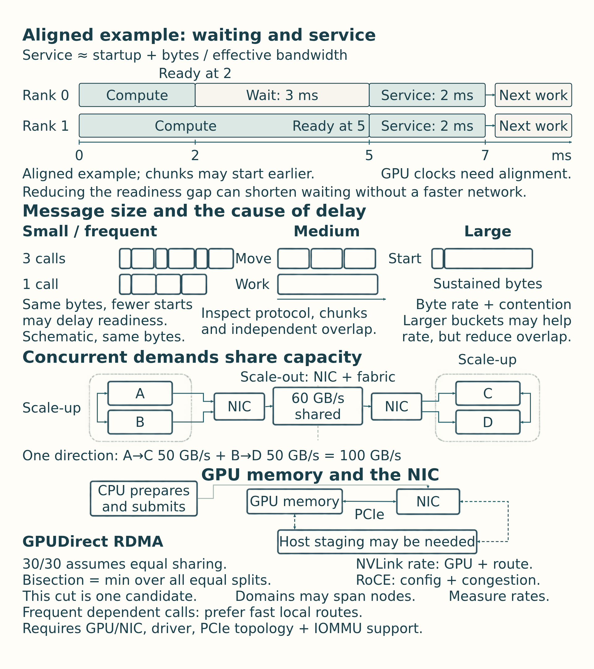
Message size changes which term dominates. A small collective can be slow because every rank pays startup and synchronization cost. A very large collective can use the fabric efficiently but spend most of its time moving bytes. Middle sizes are often the hardest to reason about because protocol choice, chunking, queueing, and overlap determine whether latency or bandwidth is exposed.
| Message-size range | Dominant cost | Typical examples | Useful change |
|---|---|---|---|
| Small and frequent | Startup latency, synchronization, launch overhead, rank skew | Per-layer tensor-parallel collectives, small control tensors, frequent expert routing metadata | Reduce message count, keep traffic in the fast local domain, combine operations when possible |
| Medium | Transition between latency and bandwidth; protocol and chunking choices matter | FSDP layer all-gathers, moderate gradient buckets, activation transfers | Tune bucket or shard sizes, improve overlap, and inspect backend algorithm choice |
| Large | Effective bandwidth and topology contention | Large gradient buckets, full-parameter shards, checkpoint or bulk cache movement | Use high-bandwidth paths, hierarchical collectives, compression, or overlap with independent compute |
Message size suggests whether startup delay or sustained transfer is the first limit. The route then sets the latency and bandwidth available to that payload, including the device, switch, and node boundaries where links become shared.
16.5 Topology and communication distance
Scalable clusters use switched hierarchy: endpoints connect to local switches, and the fabric routes traffic through switch layers rather than requiring every device pair to have a dedicated cable.
Large clusters often use hierarchical switch designs such as leaf-spine topologies. Leaf switches connect servers in a rack or local group. Spine switches connect leaf groups. The relevant capacity is the bandwidth available when many endpoints communicate across those groups at once.
Bisection bandwidth: The minimum aggregate bandwidth across a division of the network’s endpoints into two equal-sized groups, taking the minimum over all such divisions.4 The direction convention matters: the example below counts traffic in one direction, without adding the reverse direction’s capacity.
Example: Concurrent traffic across a network division
Suppose endpoints A and B are on one side and C and D on the other. A sends to C at 50 GB/s while B sends to D at 50 GB/s. The simultaneous demand across this division is 50 + 50 = 100 GB/s. If the paths share a 60 GB/s upstream limit, their combined rate cannot exceed 60 GB/s, even if each endpoint has a 100 GB/s link. An equal allocation would give each transfer 30 GB/s, although actual sharing depends on routing and scheduling.
Conclusion: One fast endpoint link does not establish sufficient capacity across the division. A leaf-spine design can add parallel paths as the cluster grows, but its achieved capacity depends on uplink provision and concurrent traffic. Section 17.4 connects this constraint to placement and oversubscription (upstream links with less capacity than the endpoints attached below them).
Every extra switch hop adds latency, and shared links can become congested even in a scalable switched design.
Scale-up communication stays inside a tightly coupled accelerator domain with fast GPU-to-GPU paths. That domain is often one server, but rack-scale NVLink systems can join GPUs across more than one compute tray or node. Scale-out communication crosses the cluster network through network interface cards (NICs) and fabrics such as InfiniBand, RDMA over Converged Ethernet (RoCE), or Ethernet. Frequent latency-sensitive traffic such as tensor-parallel collectives should remain inside the fastest available scale-up domain whenever possible.
A direct full mesh is the contrasting limit: every device connects to every other device. Port and cable demand grows rapidly with device count, which is why large systems use switched hierarchy instead.
\[ \text{full-mesh links} = \frac{N(N - 1)}{2} \tag{16.3}\]
A full mesh among N endpoints needs N(N - 1)/2 undirected links, so direct wiring grows quadratically. Leaf-spine fabrics replace those dedicated pairwise links with shared switch paths. A host-to-host path can be counted by switches or by physical links. State the convention before describing a path as a particular number of hops.
16.6 Rank skew and waiting
An apparently slow collective can include time spent waiting for another rank before useful transfer finishes. Four quantities help explain the interval: operation startup, the byte rate of the selected path, the topology crossed, and differences in rank readiness. Rank skew: A difference in when participating ranks become ready for the same operation. Section 16.4 estimates startup plus transfer service once the required inputs are ready. Its equation does not estimate the preceding wait for a late rank.
In an illustrative aligned two-rank timeline, rank 0 enters at 2 ms, rank 1 at 5 ms, and both finish at 7 ms. Rank 0 observes 5 ms, of which 3 ms is waiting and 2 ms is service. Real chunked collectives can overlap partial progress, so aligned traces are needed to attribute a measured delay.
Example: Rank waiting and transfer service
Assume two GPU timelines have been aligned to a common time origin. Rank 0 has its input ready and reaches the collective at 2 ms. Rank 1 reaches it at 5 ms. For this illustrative serialized schedule, no useful transfer occurs until 5 ms, and the result becomes available to both ranks at 7 ms. Dependent computation can then start at 7 ms.
Rank 0’s observed entry-to-result interval is 7 - 2 = 5 ms: 3 ms waiting plus 2 ms of collective service. Rank 1 observes 7 - 5 = 2 ms. If startup is 0.02 ms and the modeled per-rank payload is 0.198 GB over an effective 100 GB/s path, the estimate is 0.02 + 1000 x 0.198 / 100 = 2 ms. It models the service interval here, not rank 0’s full 5 ms.
Conclusion: Removing the readiness gap shortens rank 0’s observed collective interval without increasing network bandwidth. These are assumed trace values, not measurements. Real chunked collectives can make partial progress before every rank arrives, so waiting and transfer need not form two separate additive intervals. A local CUDA event pair also does not establish a shared clock across GPUs. Aligned rank traces and dependencies are needed to attribute the delay.
Optimizations target different ingredients. Larger buckets can improve bandwidth efficiency but may reduce overlap. Topology-aware rank placement can keep frequent collectives on fast links. Reducing message count can help latency-bound paths. Removing rank imbalance can shorten apparent collective time without changing the network.
Once the trace separates startup, transfer, and rank waiting, map the slow interval to the actual GPU-to-GPU or GPU-to-NIC path. The fabric and device placement determine which changes can improve it.
16.7 Physical communication paths
Communication fabrics should be described by scope. Some links move bytes inside a server. Some connect servers. Some are general-purpose and some are designed for high-performance GPU communication.
Section 3.5 defines PCIe, NVLink, NVSwitch, InfiniBand, RoCE, and Ethernet. Two of their properties matter once traffic is collective. The pairwise bandwidth of NVLink depends on the GPU model and on whether the selected GPUs are joined directly or through NVSwitch. RoCE performance depends strongly on network configuration, congestion control, and near-lossless behavior, and standard Ethernet paths are often a poor fit for frequent latency-sensitive collectives unless engineered for that workload.
- GPUDirect RDMA: Lets a compatible NIC directly access GPU memory over PCIe instead of staging the payload through host memory, following the NVIDIA GPUDirect RDMA Documentation5. The CPU still prepares and submits the communication. Direct access removes a copy path, not all CPU coordination, and it requires compatible GPU, NIC, driver, PCIe topology, and IOMMU settings. An unsupported or poorly connected path can fall back to host staging or perform badly.
Fabric caveat
A fabric name is only the starting point for a performance estimate. Effective bandwidth depends on topology, routing, contention, message size, collective algorithm (the schedule that implements a collective, Section 16.3), and whether the software stack actually uses the intended path.
The critical distinction is local versus remote path. Frequent per-layer traffic is most viable inside a fast GPU fabric. Cross-node traffic additionally traverses a GPU-to-NIC path, a network interface, switches, and the destination path. Product names and peak bandwidth figures are generation-specific, so verify the installed topology and achieved transfer rate rather than copying a nominal number.
A collective fixes which ranks contribute and receive the result, while its algorithm and physical path set part of the cost. The next chapter turns those choices into rank launch and measurement checks, including waits that a link-rate estimate cannot explain.
References
NVIDIA. (2026). NVIDIA Collective Communications Library Documentation (NCCL 2.32.3). NCCL documentation. The documentation at this link can change versions. Supports NCCL as the common GPU collective library implementing AllReduce, Broadcast, Reduce, AllGather, ReduceScatter, AlltoAll, Gather, Scatter, and point-to-point operations over paths including PCIe, NVLink, NVSwitch, and network interfaces. Limit: documents library behavior and configuration, not achieved bandwidth; algorithm choice depends on message size, rank count, topology, and settings such as NCCL_ALGO.↩︎
NVIDIA. (2024). NCCL Tests PERFORMANCE Documentation. Pinned commit c6eb15875f508076f3f26de4f7da3899701bc4db dated 2024-07-25 at NCCL Tests performance documentation, commit page at NCCL Tests pinned commit. Supports AllReduce bus-bandwidth correction factor 2 times (n minus 1) divided by n, and (n minus 1) divided by n for ReduceScatter and AllGather, with the AllReduce reduction described as independent of ring, tree, or other point-to-point algorithm. Limit: factor converts algorithm bandwidth to bus bandwidth and does not prove which schedule a runtime selects or what elapsed time a topology achieves.↩︎
NVIDIA. (2024). NCCL Tests PERFORMANCE Documentation. Pinned commit c6eb15875f508076f3f26de4f7da3899701bc4db dated 2024-07-25 at NCCL Tests performance documentation, commit page at NCCL Tests pinned commit. Supports AllReduce bus-bandwidth correction factor 2 times (n minus 1) divided by n, and (n minus 1) divided by n for ReduceScatter and AllGather, with the AllReduce reduction described as independent of ring, tree, or other point-to-point algorithm. Limit: factor converts algorithm bandwidth to bus bandwidth and does not prove which schedule a runtime selects or what elapsed time a topology achieves.↩︎
Bindel, D. (2015, October 6). Distributed memory: Networks and models. Cornell University, CS 5220 course notes, Network properties. Distributed memory: Networks and models. Supports the minimum-capacity equal-division definition. The four-endpoint rates in this chapter are assumed teaching inputs, not benchmark results.↩︎
NVIDIA. (2026). GPUDirect RDMA Documentation (v13.4). GPUDirect RDMA documentation. Supports direct data exchange between GPU and third-party PCIe peer such as a NIC, with address translation through the NVIDIA kernel driver, while CPU libraries prepare and submit transfers. Limit: peers must share a compatible PCIe root complex path, IOMMU must allow the mapping, and topology, BAR size, and platform support determine whether the direct path is available or falls back.↩︎