18 Replicated and sharded training
More GPUs can process different training examples at once, but each model copy still needs parameters, gradients, and optimizer state. If that full state fits on every GPU, replicated training can divide the data and synchronize gradients. When those copies exceed the memory budget, partitioning selected state across ranks can reduce persistent storage on each device.
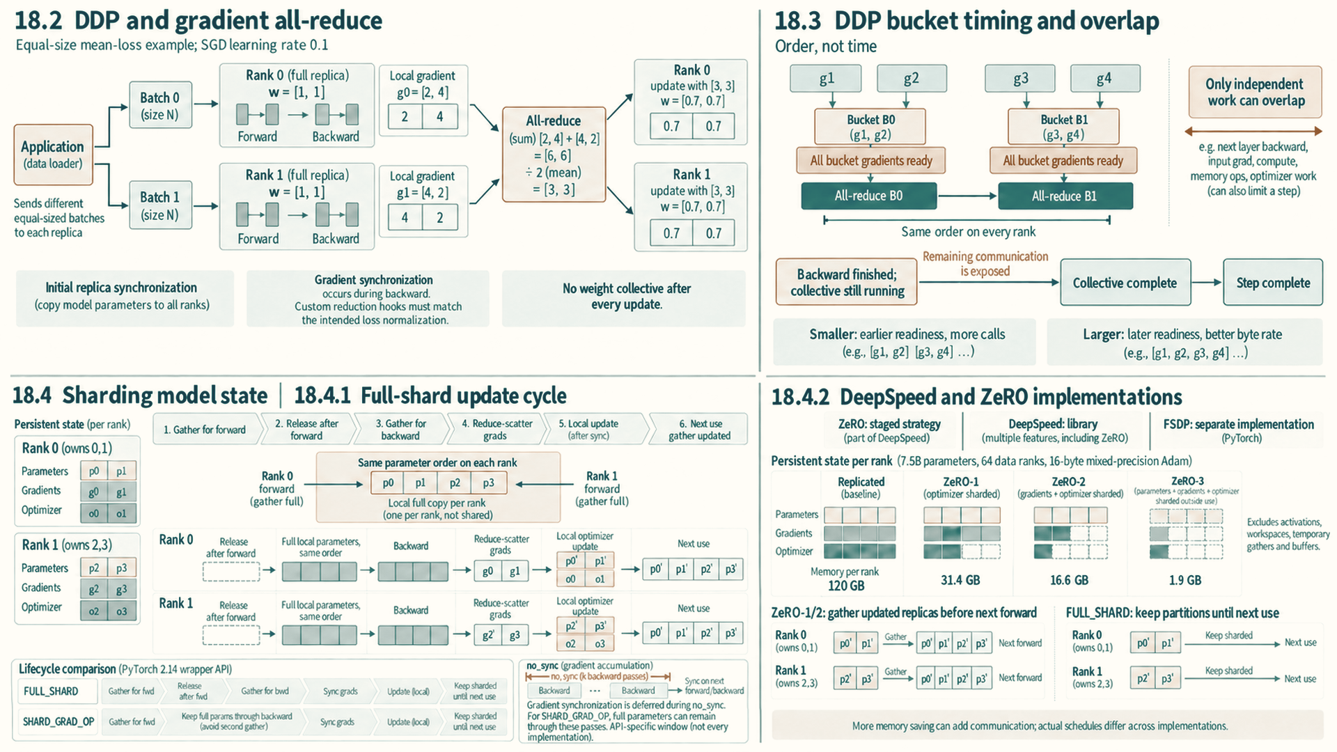
The memory saving changes the update cycle. A rank may need gathered parameters for computation, a reduced gradient shard for its local optimizer, and newly updated parameters at the next use. Temporary full tensors and communication buffers still count toward peak memory. The choice between replication and sharding therefore depends on both the live memory windows and the exchanges that remain exposed in the training step.
18.1 Work and state beyond one GPU
Scaling beyond one GPU means deciding which object is too large or too slow on one device. The answer determines the distributed strategy.
- Data: The training examples or serving requests. Splitting data can increase throughput when each replica can fit the full model, enough work is available, and communication does not dominate.
- Model state: Parameters, gradients, and optimizer state. Sharding state reduces per-GPU memory but introduces communication to gather or reduce the pieces that each step needs.
- Layer computation: Matrix multiplications and attention inside a layer. Tensor parallelism splits this work, but then partial results must be combined frequently.
- Layer sequence: The ordered stack of transformer layers. Pipeline parallelism places different layer ranges on different devices and moves activations between stages.
- Experts: Specialized modules in a Mixture-of-Experts model. Expert parallelism routes token representations to the devices where selected experts are placed.
Replication is simple but duplicates memory. Sharding saves memory or increases parallel compute, but it creates communication that must fit the topology. Distributed strategies are applications of collective communication and physical fabric constraints, not replacements for them.
The object being split determines the communication obligation: replicated models synchronize gradients, while split model work exchanges activations or partial results. The next question is how Distributed Data Parallel (DDP) turns replicated parameters and different local mini-batches into synchronized updates.
18.2 DDP and gradient all-reduce
Distributed Data Parallel (DDP) is the baseline multi-GPU training strategy when the full model fits on every GPU. Each process holds one model replica and computes local gradients on one mini-batch drawn from its assigned data shard, then synchronizes gradients before the optimizer step. DDP itself does not shard the input. The application assigns per-rank shards, for example with a distributed sampler.
PyTorch DDP is a training strategy implemented above torch.distributed. The wrapper registers gradient hooks and groups gradients into buckets with a configurable bucket_cap_mb, following the Distributed Data Parallel design note1. The process group and its backend execute the all-reduces required to keep replicas synchronized.
- Rank: The integer identity of a participating process within its process group, as defined in Section 3.4. A common setup uses one process per GPU.
- Replica: A full copy of the model parameters on one rank. DDP keeps replicas numerically synchronized by all-reducing gradients.
- Local mini-batch: The examples one rank processes in one forward and backward pass, also called its local micro-batch (Section 9.3).
- Global batch: The examples used for one optimizer update across ranks and accumulation steps. With equal per-rank counts, it is the number of examples in one local mini-batch times the number of data-parallel ranks times the number of accumulation steps.
- Gradient all-reduce: Each rank contributes gradients, the gradients are reduced, and every rank receives the same synchronized result.
DDP works well when the model fits on each GPU and synchronization takes a small enough share of each step. It does not reduce parameter memory because every rank stores a full replica. When model state is the memory wall, FSDP or another sharding strategy can reduce each GPU’s stored state.
DDP’s default initialization synchronizes replicas from rank 0. Backward hooks reduce gradient buckets, and every rank applies an equivalent optimizer update after the required synchronization. With the default reduction, DDP averages gradients across ranks. Custom communication hooks can change that reduction, so the loss normalization and reduction rule must agree.2
Default DDP synchronizes gradients during backward. It does not add a weight-synchronization collective after each optimizer step.3
The implementation pattern is one process per GPU: initialize the process group, map LOCAL_RANK to the local CUDA device, wrap the model with Distributed Data Parallel, shard the data stream with a distributed sampler, and let backward hooks launch gradient all-reduces. For one update, suppose two ranks start with parameters [1, 1] and compute local gradients [2, 4] and [4, 2] from equally sized mini-batches under a mean-loss rule. SUM all-reduce returns [6, 6] to both; division by two gives the mean gradient [3, 3]. Stochastic gradient descent (SGD) subtracts learning rate times gradient. With learning rate 0.1, it updates both replicas to [0.7, 0.7]. This trace assumes no accumulation or momentum. Matching initial parameters, synchronized gradients, and the same update rule keep the replicas equal without another weight collective.
18.3 DDP bucket timing and overlap
Section 17.2 gives the general overlap rule. In DDP, communication/computation overlap uses the order of backward propagation. Gradients for later layers become ready while earlier layers are still computing backward, so DDP can start all-reducing ready gradient buckets before the full backward pass completes.
- Gradient bucket: A group of parameter gradients packed together so DDP can launch fewer, larger all-reduces instead of one collective per tensor.
- Ready time: The moment all gradients in a bucket have been produced by backward propagation.
- Hidden communication: Communication that finishes during independent backward work, leaving no exposed tail from that exchange. Contention for shared resources can still lengthen the step (Section 17.2).
- Exposed tail: The communication left after the last useful computation has finished (Section 9.1). Here it is the part of the gradient all-reduce that no backward work covers.
Overlap has a cost. Small buckets may start earlier while reducing bandwidth efficiency because there are more collectives. Large buckets may use bandwidth better while starting later and leaving a larger exposed tail. The useful measurement is whether reducing collective time would still reduce the end-to-end training step.
The DDP reducer turns many parameter gradients into bucket-level communication. A bucket becomes ready when all its gradients are available, but reductions must launch in the same bucket order on every rank. A ready bucket can therefore wait for an earlier bucket. Once that ordering condition is met, its reduction can run while earlier layers in the backward pass are still computing.4
Bucket setup and the timing of one update can be read in this order:
- Form the buckets: Group parameter gradients using a configured limit such as
bucket_cap_mb. Smaller buckets can start earlier. Larger buckets usually use bandwidth more efficiently. - Mark gradients ready: Autograd hooks mark each parameter gradient as backward propagation produces it. Parameter order and graph structure determine when every gradient in a bucket is available.
- All-reduce launch: A ready bucket is reduced in the shared bucket order across the data-parallel ranks, usually through NCCL on NVIDIA GPUs. The communication overlaps only while independent backward computation continues.
- Exposed tail: Communication remaining after backward computation finishes directly lengthens the training step.
A slow DDP step can still come from local causes such as data loading, forward kernels, backward memory pressure, or optimizer state. Distributed causes add rank skew, all-reduce bandwidth, bucket timing, and topology placement.
18.4 Sharding model state
Fully Sharded Data Parallel (FSDP) supports several sharding strategies. Under FULL_SHARD, parameters, gradients, and optimizer state are sharded across ranks outside their materialized use windows, following the FullyShardedDataParallel documentation5. Other strategies replicate or retain more state. Full sharding reduces per-GPU memory but introduces parameter all-gather and gradient reduce-scatter around layer execution.
18.4.1 Full-shard update cycle
Full sharding has separate forward and backward communication phases. Parameters are all-gathered before forward computation and may be resharded afterward. If forward released the full parameters, they are gathered again before backward computation. As gradients become ready, reduce-scatter combines them and leaves each rank with its local shard. Prefetch settings can overlap a future gather with current computation, but they may raise peak memory by materializing parameters earlier.
One full-shard layer follows this communication sequence:
- Gather before forward: All-gather parameter shards so the layer can compute. Prefetching too early increases peak memory.
- Reshard after forward: Release or reshard the full parameters according to the selected strategy. Keeping them improves reuse but reduces memory savings.
- Gather before backward: All-gather parameters again when forward released them. Backward prefetch can overlap this transfer with compute while increasing live memory.
- Reduce after gradients are ready: Reduce-scatter gradients and retain each rank’s local shard. Communication that remains after compute becomes the exposed tail.
- Update the local parameter shard: Once the step’s required backward, accumulation, and synchronization are complete, each rank’s optimizer uses its reduced gradient shard and matching optimizer-state shard to update the same parameter indices. This is one step update, not a separate update each time a layer finishes backward.
- Gather updated values at next use: Full sharding keeps the updated parameter partitions on their ranks. The next forward gathers those new partitions when the wrapped unit is needed. Optimizer buffers remain local.6
A concrete optimizer update makes the final stage of the sharded cycle visible. Stochastic gradient descent (SGD) with momentum is an optimizer that keeps a decaying sum of past gradients and moves parameters against that accumulated direction. Its momentum buffer stores that history for each parameter between steps. The example uses this shorter update rule to expose how parameter, gradient, and optimizer-state shards stay aligned.
Example: From gradient shards to updated parameters
Consider one four-parameter unit in a training step after momentum buffers have already been initialized. Rank 0 stores parameters \([1,2]\) and momentum \([0.5,-0.5]\) for indices 0 and 1. Rank 1 stores parameters \([3,4]\) and momentum \([1,-1]\) for indices 2 and 3. A forward all-gather temporarily supplies \([1,2,3,4]\) on both ranks. If full parameters are released after forward, a second gather reconstructs the same values for backward. Parameters stay unchanged until the step update.
Suppose backward on equally weighted local data shards produces gradient contributions [1, 2, 3, 4] and [3, 6, 9, 12]. SUM reduce-scatter followed by division by two leaves rank 0 with mean-gradient shard [2, 4] and rank 1 with [6, 8]. The division expresses this example’s mean-loss convention, not an implicit property of SUM.
The momentum SGD update is \(v' = 0.9v + g\) followed by \(p' = p - 0.1v'\), where \(p\) is a parameter shard, \(g\) its mean-gradient shard, and \(v\) its existing momentum buffer. The prime denotes the new value. The factor 0.9 retains part of the previous buffer, and the learning rate 0.1 sets the parameter change per unit of new momentum. This omits weight decay, dampening, and Nesterov momentum.7
| Rank | New momentum, 0.9v + g | New parameters, p - 0.1v’ |
|---|---|---|
| 0 | \([0.45+2,-0.45+4]=[2.45,3.55]\) | \([1-0.245,2-0.355]=[0.755,1.645]\) |
| 1 | \([0.9+6,-0.9+8]=[6.9,7.1]\) | \([3-0.69,4-0.71]=[2.31,3.29]\) |
The next forward all-gather supplies [0.755, 1.645, 2.31, 3.29] on both ranks. Each rank retains only its own updated parameter and momentum partitions between full-shard use windows. Adam would retain two moment buffers per parameter and use a different update rule, but the matching of local parameter, gradient, and optimizer-state indices is the same.
Conclusion: Gradient reduction is followed by a local update and later parameter materialization. Persistent shards and temporary full tensors occupy different storage windows. The values here illustrate that cycle, not measured convergence or runtime performance.
In PyTorch 2.14’s FullyShardedDataParallel API, FULL_SHARD gathers a wrapped unit’s parameters before forward, reshards afterward, gathers again for backward, and reshards after backward. SHARD_GRAD_OP gathers before forward but keeps those full parameters through backward, then reshards them. Both keep optimizer state partitioned and reduce-scatter gradients on synchronized steps. Retaining full parameters removes the second gather but lengthens their memory lifetime. FSDP’s no_sync() context defers gradient synchronization during accumulation. FSDP retains full gradients instead of gradient shards until synchronization, so peak memory can rise substantially. The first forward-backward pass after leaving the context synchronizes the accumulated gradients. Inside this context, SHARD_GRAD_OP also retains full parameters after backward. These windows refer to the cited ShardingStrategy API, not every API called FSDP.8
18.4.2 DeepSpeed and ZeRO implementations
Zero Redundancy Optimizer (ZeRO) names the staged sharding strategy, following ZeRO: Memory Optimizations Toward Training Trillion Parameter Models9, while DeepSpeed is a distributed-training library that implements ZeRO-family state placement together with optimizer, pipeline, and runtime integrations. PyTorch FSDP provides built-in sharding strategies within PyTorch. Its FULL_SHARD mode partitions parameters, gradients, and optimizer state.
The choice between these implementations follows the required state placement and collective schedule. Configuration names differ, but memory savings and communication costs follow the same parameters, gradients, optimizer state, all-gather, and reduce-scatter objects.
PyTorch FSDP and DeepSpeed ZeRO Stage 3 are related full-sharding approaches with similar state-placement goals, but they are distinct APIs and implementations with different policies and scheduling behavior. The comparison below therefore follows the parameter, gradient, and optimizer-state lifecycle instead of treating the implementations as interchangeable.
The ZeRO family names three progressively broader state-sharding choices:
- ZeRO-1: Shards optimizer state while parameters and gradients remain replicated. The 16 bytes per parameter of Section 2.1 become \(4+12/N_d\) bytes per rank, where \(N_d\) is the number of data-parallel ranks and 12 bytes are the optimizer’s FP32 master copy and two Adam moments.
- ZeRO-2: Also shards gradients, leaving \(2+14/N_d\) bytes per parameter per rank. Reduce-scatter timing follows bucket readiness, hooks, overlap, and implementation policy rather than an unconditional immediate layer-by-layer rule.
- ZeRO-3: Also shards parameters outside their materialized use windows, leaving \(16/N_d\) bytes per parameter per rank. Implementations may reshard or retain gathered parameters. Temporary full parameters and communication buffers still consume memory.
Example: Model-state memory per GPU under ZeRO
Inputs: The ZeRO paper’s example model has \(7.5\times10^9\) parameters trained with mixed-precision Adam on \(N_d=64\) data-parallel GPUs.10 Activations, workspaces, and buffers are excluded.
| Stage | Bytes per parameter per GPU | Model state per GPU |
|---|---|---|
| Plain data parallelism | 16 | 120 GB |
| ZeRO-1 | \(4+12/64\approx4.19\) | 31.4 GB |
| ZeRO-2 | \(2+14/64\approx2.22\) | 16.6 GB |
| ZeRO-3 | \(16/64=0.25\) | 1.9 GB |
Conclusion: Most of the saving comes from the optimizer state, which is 12 of the 16 bytes. At 64 ranks, sharding the gradients as well reduces 31.4 GB to 16.6 GB, nearly halving what remains. Sharding the parameters makes this persistent model-state estimate fall in proportion to the number of GPUs. The price is communication: ZeRO-3 gathers parameters before they are used, which the paper puts at about 1.5 times the communication volume of plain data parallelism under its communication model.
The comparison below holds the data-parallel goal fixed and shows which model-state objects remain replicated or become sharded. The final column identifies the communication phase introduced by each broader sharding choice.
| Strategy | Parameters | Gradients | Optimizer state | Main timing cost |
|---|---|---|---|---|
| DDP | Replicated | All-reduced and replicated | Replicated | Gradient all-reduce after buckets become ready |
| ZeRO-1 | Replicated | Replicated | Sharded | Gradient synchronization, local partition update, then distribution of updated parameter partitions to all replicas |
| ZeRO-2 | Replicated | Reduce-scattered or sharded | Sharded | Gradient reduce-scatter, local partition update, then distribution of updated parameter partitions to all replicas |
| ZeRO-3 / FSDP FULL_SHARD | Sharded outside layer execution | Reduce-scattered and sharded | Sharded | Parameter all-gather before forward/backward layer use plus reduce-scatter after gradients |
ZeRO-1 and ZeRO-2 also let each rank update its assigned parameter partition using local optimizer state. They then distribute the updated partitions, for example by all-gather, to restore the full parameter replicas before the next forward. In the example, each replica must receive both [0.755, 1.645] and [2.31, 3.29]. ZeRO-1 keeps the synchronized gradients replicated, whereas ZeRO-2 partitions them as well. Full sharding instead leaves parameters partitioned between their next-use gathers.11
When even sharded model state does not fit, selected state can move to host memory. Offload stores that state on the CPU and transfers the values needed by GPU computation. ZeRO-Offload runs optimizer computation on the CPU. The paper also describes an optional one-step delayed update that overlaps CPU optimizer work with GPU computation. This changes which step’s gradients supply the update. In its tested V100 setup, the authors report training models with over 13 billion parameters on one GPU, about ten times their PyTorch baseline, without model changes.12 PyTorch FSDP’s CPUOffload option keeps parameters on the CPU when they are not in use, which also moves the gradients to the CPU and runs the optimizer step there.13 Offload trades GPU memory for PCIe traffic (Section 3.4) and CPU optimizer time. It is useful when the capacity gain outweighs those costs for the workload.
Full sharding reduces persistent per-rank model state by adding timed parameter gathers and gradient reduce-scatters. Its benefit depends on peak-memory relief compared with exposed communication and temporary materialization. When state sharding alone cannot meet the target, tensor and sequence parallelism (Chapter 19) asks whether to split layer work or long-context state. Pipeline and expert layouts (Chapter 20) then follow work across layer stages and remote experts.
References
PyTorch. (2026). Distributed Data Parallel. Versioned v2.14 design note at Distributed Data Parallel design note, created 2026-05-16 and updated 2026-05-16, describing implementation state as of v1.4. Supports Reducer gradient buckets with
bucket_cap_mb, autograd hooks, per-bucket async all-reduce with mean gradients, same-order all-reduce across ranks, and overlap of collectives with backward compute. Limit: input sharding is done by the application, for example with a distributed sampler; DDP synchronizes gradients but does not partition inputs by itself.↩︎PyTorch. (2026). Distributed Data Parallel. Versioned v2.14 design note at Distributed Data Parallel design note, created 2026-05-16 and updated 2026-05-16, describing implementation state as of v1.4. Supports Reducer gradient buckets with
bucket_cap_mb, autograd hooks, per-bucket async all-reduce with mean gradients, same-order all-reduce across ranks, and overlap of collectives with backward compute. Limit: input sharding is done by the application, for example with a distributed sampler; DDP synchronizes gradients but does not partition inputs by itself.↩︎PyTorch. (2026). Distributed Data Parallel. Versioned v2.14 design note at Distributed Data Parallel design note, created 2026-05-16 and updated 2026-05-16, describing implementation state as of v1.4. Supports Reducer gradient buckets with
bucket_cap_mb, autograd hooks, per-bucket async all-reduce with mean gradients, same-order all-reduce across ranks, and overlap of collectives with backward compute. Limit: input sharding is done by the application, for example with a distributed sampler; DDP synchronizes gradients but does not partition inputs by itself.↩︎PyTorch. (2026). Distributed Data Parallel. Versioned v2.14 design note at Distributed Data Parallel design note, created 2026-05-16 and updated 2026-05-16, describing implementation state as of v1.4. Supports Reducer gradient buckets with
bucket_cap_mb, autograd hooks, per-bucket async all-reduce with mean gradients, same-order all-reduce across ranks, and overlap of collectives with backward compute. Limit: input sharding is done by the application, for example with a distributed sampler; DDP synchronizes gradients but does not partition inputs by itself.↩︎PyTorch. (2026). FullyShardedDataParallel,
ShardingStrategyentries. Versioned v2.14 documentation at FullyShardedDataParallel documentation, created 2022-02-02 and updated 2026-05-12. Supports theFULL_SHARDandSHARD_GRAD_OPstorage windows, gathers, gradient reduce-scatter, and local optimizer updates described here.SHARD_GRAD_OPretains full parameters after backward insideno_sync(). Limit: this wrapper’s API contract does not establish the behavior of every FSDP API or achieved step time.↩︎PyTorch. (2026). FullyShardedDataParallel,
ShardingStrategyentries. Versioned v2.14 documentation at FullyShardedDataParallel documentation, created 2022-02-02 and updated 2026-05-12. Supports theFULL_SHARDandSHARD_GRAD_OPstorage windows, gathers, gradient reduce-scatter, and local optimizer updates described here.SHARD_GRAD_OPretains full parameters after backward insideno_sync(). Limit: this wrapper’s API contract does not establish the behavior of every FSDP API or achieved step time.↩︎PyTorch. (2026). SGD. Versioned v2.14 API documentation at SGD API documentation. Supports the momentum-buffer recurrence and parameter update. The illustration assumes existing buffers and excludes weight decay, dampening, and Nesterov momentum. It does not illustrate Adam’s update or distributed optimizer implementation details.↩︎
PyTorch. (2026). FullyShardedDataParallel,
ShardingStrategyentries. Versioned v2.14 documentation at FullyShardedDataParallel documentation, created 2022-02-02 and updated 2026-05-12. Supports theFULL_SHARDandSHARD_GRAD_OPstorage windows, gathers, gradient reduce-scatter, and local optimizer updates described here.SHARD_GRAD_OPretains full parameters after backward insideno_sync(). Limit: this wrapper’s API contract does not establish the behavior of every FSDP API or achieved step time.↩︎Rajbhandari, S., Rasley, J., Ruwase, O., & He, Y. (2020). ZeRO: Memory Optimizations Toward Training Trillion Parameter Models. Preprint at ZeRO paper (DOI), v2 submitted 2019-10-07, v3 revised 2020-05-13. Supports staged sharding with Stage 1 for optimizer states, Stage 2 adding gradients, and Stage 3 adding parameters outside materialized use windows. The paper gives per-rank model-state memory of 4 + K/N_d, 2 + 14/N_d, and 16/N_d bytes per parameter with K = 12, the 7.5B-parameter, 64-GPU example of 120, 31.4, 16.6, and 1.9 GB, and a 1.5x communication volume for parameter partitioning. Limit: memory and scaling results depend on model, device count, and implementation policy for gathering and resharding.↩︎
Rajbhandari, S., Rasley, J., Ruwase, O., & He, Y. (2020). ZeRO: Memory Optimizations Toward Training Trillion Parameter Models. Preprint at ZeRO paper (DOI), v2 submitted 2019-10-07, v3 revised 2020-05-13. Supports staged sharding with Stage 1 for optimizer states, Stage 2 adding gradients, and Stage 3 adding parameters outside materialized use windows. The paper gives per-rank model-state memory of 4 + K/N_d, 2 + 14/N_d, and 16/N_d bytes per parameter with K = 12, the 7.5B-parameter, 64-GPU example of 120, 31.4, 16.6, and 1.9 GB, and a 1.5x communication volume for parameter partitioning. Limit: memory and scaling results depend on model, device count, and implementation policy for gathering and resharding.↩︎
Rajbhandari, S., Rasley, J., Ruwase, O., & He, Y. (2020). ZeRO: Memory Optimizations Toward Training Trillion Parameter Models. Preprint at ZeRO paper (DOI), v2 submitted 2019-10-07, v3 revised 2020-05-13. Supports staged sharding with Stage 1 for optimizer states, Stage 2 adding gradients, and Stage 3 adding parameters outside materialized use windows. The paper gives per-rank model-state memory of 4 + K/N_d, 2 + 14/N_d, and 16/N_d bytes per parameter with K = 12, the 7.5B-parameter, 64-GPU example of 120, 31.4, 16.6, and 1.9 GB, and a 1.5x communication volume for parameter partitioning. Limit: memory and scaling results depend on model, device count, and implementation policy for gathering and resharding.↩︎
Ren, J., Rajbhandari, S., Aminabadi, R. Y., Ruwase, O., Yang, S., Zhang, M., Li, D., & He, Y. (2021). ZeRO-Offload: Democratizing Billion-Scale Model Training. USENIX ATC 2021. arXiv:2101.06840. Supports offloading data and compute to the CPU, a fast CPU optimizer whose step can overlap GPU compute through a one-step delayed parameter update, and training models with over 13 billion parameters on a single GPU, a 10x increase over PyTorch, without model changes. Limit: throughput depends on CPU speed and PCIe bandwidth.↩︎
PyTorch. (2026). FullyShardedDataParallel,
CPUOffload(v2.14 documentation). FSDP CPUOffload documentation. Supports thatoffload_params=Trueoffloads parameters to the CPU when they are not involved in computation, which also offloads gradients so that the optimizer step runs on the CPU. Limit: the page documents behavior, not the resulting step time.↩︎