15 Serving measurement and stack selection
A busy GPU can still leave users waiting. A request may spend time in a queue, wait for its first token, or receive later tokens too slowly. The service also has to account for rejected requests and work that remains unfinished. Request traces and outcome counts show whether a configuration delivers useful completed work within the latency and quality targets.
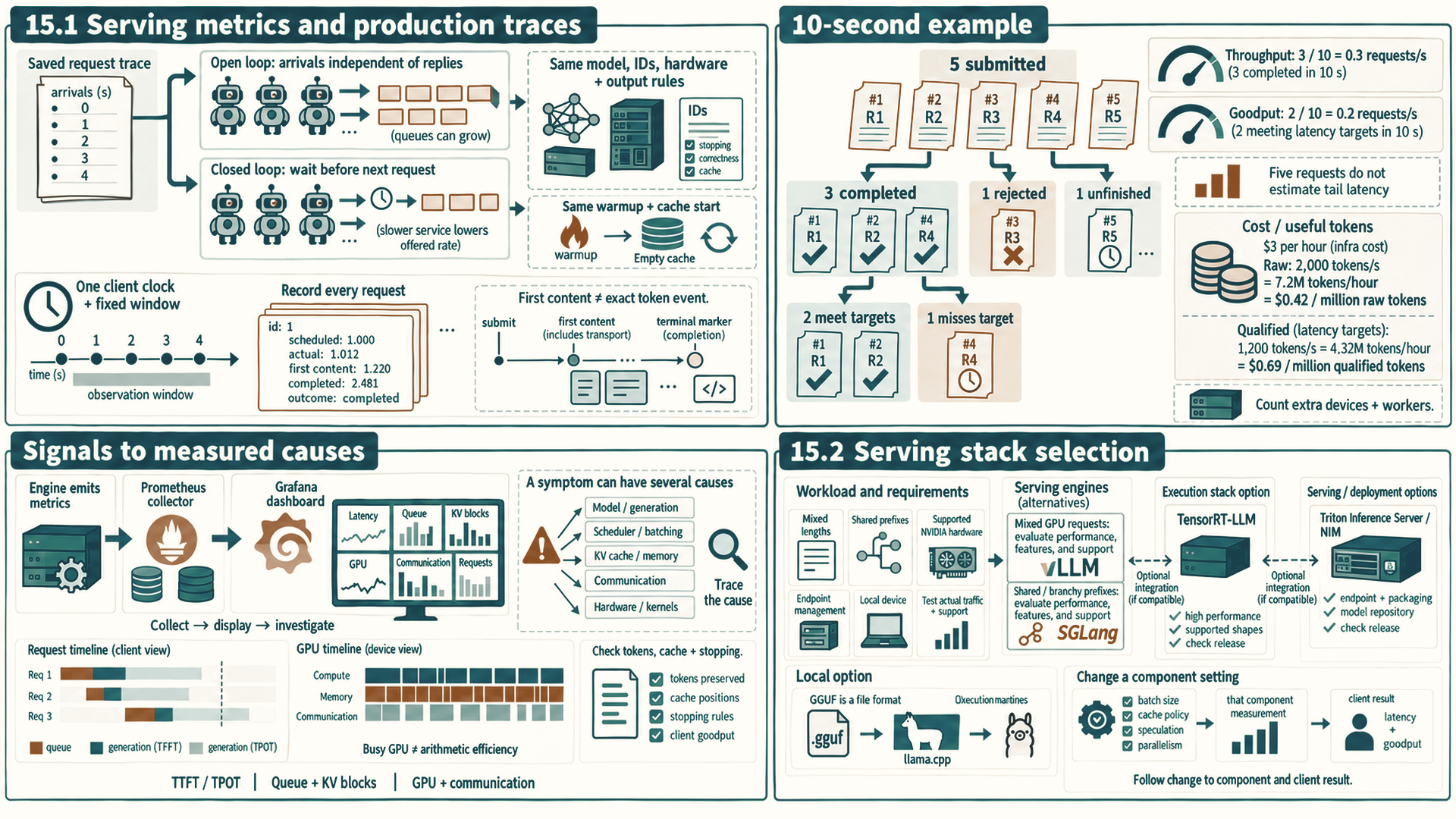
That evidence also guides the software choice. A stack must support the intended model and hardware, manage the workload’s batching and cache needs, and fit the deployment’s preparation and operating requirements. Production metrics locate a symptom; a controlled comparison tests whether a proposed change improves it. Peak throughput from one fixed shape cannot answer both questions for a service with varying prompts, outputs, and arrivals.
15.1 Serving metrics and production traces
The production monitoring system collects measurements from the serving engine. The engine exposes metrics from its scheduler, request queue, token loop, cache manager, and GPU worker processes. A metrics collector stores those time series, and a dashboard turns them into views an operator can inspect during incidents or capacity planning.
Prometheus is commonly used as the metrics collector: it scrapes HTTP endpoints exported by services and stores numeric time series. Grafana is commonly used as the dashboard layer: it queries Prometheus and displays latency, throughput, queueing, cache, and utilization trends. These tools do not optimize inference by themselves. They make the effects of scheduling and cache policy visible. A dashboard’s GPU-utilization panel usually shows the fraction of time a kernel is running, not how much of the GPU’s arithmetic is used (quantities and formulas, Section 6.3), so a busy decode fleet can show nearly 100 percent while it is memory-bound.
Chapter 10 defines the request-timing conventions for TTFT, inter-token latency, TPOT, end-to-end latency, throughput, and goodput. This section reuses those measures to locate a production symptom. The measures do not prove one cause by themselves, because queueing, kernels, memory, scheduling, and communication can affect the same latency measurement.
- Time To First Token (TTFT): Measures elapsed time until the first generated token. High TTFT can come from queueing, tokenization, prefix-cache misses, prefill work, communication, or cold setup. Use traces to separate them.
- Time Per Output Token (TPOT): Measures average decode time per generated token under the stated convention. Spikes can come from memory traffic, launch gaps, scheduler work, preemption, communication, or competing prefill.
- Queue Time: Measures the time requests spend waiting in the scheduler before admission. Use it to check whether waiting for admission contributes to high TTFT or end-to-end latency.
- KV cache utilization: Tracks occupied cache blocks or bytes under the engine’s definition. High use may reflect useful admission or inefficient retention. Approaching the configured limit can cause waiting, eviction, recomputation, or preemption depending on policy.
A service comparison also needs a request-arrival contract. With open-loop load, request times are fixed independently of replies, so a slow service can build a queue. With closed-loop load, each client waits for its reply before submitting again, so a slower response also lowers the offered request rate. These policies test different operating points even when prompt lengths match.
A fair service comparison holds the model, tokenizer, hardware, prompt and output rules, arrival policy, cache starting state, and observation window fixed while changing the serving setting being tested. Report all submitted outcomes, including rejected and unfinished requests. Completed-request throughput counts completed requests per elapsed time; goodput counts only correct completed requests meeting the predeclared latency targets in the same window.
Example: A fixed request-load comparison
This illustrative trace compares baseline and candidate serving settings in inference mode with the same loaded model, tokenizer, hardware, prompt IDs, output rules, and correctness check. It is an experiment design with invented timestamps, not a measured benchmark.
The saved request sequence contains R1 through R5 in that order, with exact prompt texts (Return only the digit 1., Return only the digit 2., Return only the digit 1., Return only the digit 2., Return only the digit 1.). The same pinned tokenizer and chat template produce each request’s token IDs and lengths, which are saved before either run. Each request asks for at most eight output tokens with greedy selection and the same EOS policy. Correctness means the stripped returned text equals the requested digit. The generator submits the requests at 0, 1, 2, 3, and 4 seconds without waiting for responses. It permits five outstanding requests, enough to submit this whole trace even if none finishes. If the generator misses a scheduled arrival, the run is invalid for this comparison. Actual submission times are recorded alongside scheduled times.
Compilation and allocator warmup finish before time zero. Each run then starts with an empty reusable prefix cache and no active requests. Warmup cache entries are cleared and that empty state is checked. Reuse within the five-request trace is allowed. The same policy applies to both settings. A separate warm-cache experiment would need the same saved priming requests before both runs.
The observation window is [0, 10] seconds on the load generator’s monotonic clock. Arrival means client submission. For this trace, first-token timing means the first generated content received by that same client, as collected below; completion is receipt of the terminal stream marker. These measurements include transport and use the same client convention in both runs. There are no retries. Rejected requests, failed streams, and requests still unfinished at 10 seconds remain in the outcome counts. Unfinished requests are canceled after the window and the engine is drained before the next run.
Suppose R1 has TTFT 0.2 seconds and completes at 1 second, R2 has TTFT 0.4 seconds and completes at 2.5 seconds, R3 is rejected, R4 has TTFT 0.8 seconds and completes at 6 seconds, and R5 is unfinished at 10 seconds. The predeclared objective requires a correct completed response, TTFT at most 0.5 seconds, and end-to-end latency at most 2 seconds. Assume the three completed outputs pass the fixed correctness check.
R1 and R2 meet the objective: their end-to-end times are 1 - 0 = 1 and 2.5 - 1 = 1.5 seconds. R4 takes 6 - 3 = 3 seconds and also misses the TTFT limit. The totals are five submitted, three completed, one rejected, and one unfinished. Completed-request throughput is 3 / 10 = 0.3 requests/s. Goodput is 2 / 10 = 0.2 requests/s, with two of five submitted requests meeting the objective. Rejected and unfinished requests contribute no successful work. Completed-request latency statistics retain R4 and report their three-request sample size, alongside the other outcome counts.
The same trace and ten-second window apply to the candidate. Changing only the serving setting makes differences interpretable. Repeated runs and a longer representative trace are needed for reliable tail estimates. Five requests demonstrate the accounting, not p95 or p99 performance.
Collecting the client trace: The following procedure turns that design into a request record. Start with an already running compatible streaming endpoint, its model name and access settings, the five saved prompts, and the selected engine’s documented warmup/cache reset. For example, a vLLM chat endpoint accepts /v1/chat/completions requests with messages and stream=true; the engine’s release determines the supported request fields.1 Use an event-aware HTTP client that can send this request and yields each complete event’s data as a string, without the data: field prefix or event delimiters. It handles events split across transport reads and multiple events in one read. Confirm one request returns usable text before preparing both runs.
- Prepare one identical request body per prompt, using the pinned chat template and model, greedy selection, the same EOS policy, and at most eight output tokens. Enable streaming. For a compatible chat endpoint, the prompt is the user content in
messages, withtemperature=0,max_tokens=8, andstream=true. Check these fields against the chosen release. Finish warmup and establish the stated cache starting state before the observation window. - Set time zero from
time.perf_counter()on the load generator. Use independent asynchronous request workers, with a five-request outstanding limit, to initiate the five HTTP calls at offsets 0, 1, 2, 3, and 4 seconds. Each worker records its actual submission-attempt time immediately before initiating its request. Do not wait for one response before starting the next request. Choose an allowed scheduling lateness before both runs; recordactual - scheduledfor every request and invalidate a run that exceeds it. - Read complete event-data strings from that client as the response arrives. Check for the terminal string
[DONE]before JSON parsing. Treat it as completion, not as another content record. Parse the other event-data strings as JSON and append nonemptychoices[0].delta.contenttext when a choice is present. Ignore role-only, usage-only, or empty-content records for the first-content timestamp. Record the first-content timestamp when the client delivers its first event with nonempty generated text, and completion when it delivers the terminal event. A stream that closes without its expected completion marker is recorded as failed. A JSON record carrying an error also marks the request failed, even if the HTTP status was successful. An event or transport read can contain several tokens, so this gives client first-content latency, not an individual-token ITL trace. Use engine token events when exact per-token timing is needed. - Save one row per submitted request: request ID, scheduled and actual submission time, first-content time or missing value, completion time or missing value, outcome, returned text, and correctness result. HTTP refusal is a rejection; a failed or disconnected stream is recorded as failed. At ten seconds, mark still-active requests unfinished, cancel their client tasks, and drain the engine before the next run. No retry enters this comparison. Compute completed throughput and goodput from the same window, retaining every submitted outcome.
For a serving change, also check that generated tokens, cache positions, and stopping or constrained-decoding behavior remain correct. Report latency and throughput together because a scheduler can improve one while harming the other. GPU event time measures device-stream work; this client record also includes submission, queueing, transport, and incomplete outcomes.
All times above use seconds relative to the same client clock. Compare client first-content latency with the matching baseline convention; do not substitute a server’s first-token emission time. The trace establishes observable request behavior. GPU traces and engine metrics are still needed to explain its cause.
Production traces connect these service symptoms to components. Poor decode throughput calls for request-admission, batch, cache-allocation, prefix-reuse, scheduler-limit, and TPOT records. High TTFT calls for separate tokenization, queue, prefill, and cache-setup intervals. A high service metric alone cannot identify a slow kernel.
The service-level measure that operators and product owners share is cost per generated token. It follows from the same quantities: the hourly cost of the GPUs divided by the tokens they deliver per hour at the latency target.
Example: Cost per million tokens
Inputs: One GPU costs an illustrative $3 per hour and sustains 2,000 generated tokens per second at the tested load, before filtering by the latency target.
Calculation: One hour delivers \(2{,}000\times3{,}600=7.2\) million tokens, so the cost is \(3/7.2\approx\$0.42\) per million tokens. If only 1,200 tokens per second meet the latency target, because pushing throughput higher breaks TPOT, the goodput-based cost is \(3/(1{,}200\times3{,}600/10^6)\approx\$0.69\) per million tokens.
Conclusion: Cost per token uses goodput, not peak throughput. Every lever that raises the tokens served within the SLO, such as batching, model compression for inference (Chapter 11), prefix caching, or speculative decoding, lowers this GPU cost per token by the same factor only if hourly GPU cost stays fixed. Additional draft-model devices, extra workers, or other serving costs must be included when they change.
A practical serving dashboard should group metrics by the subsystem that owns the symptom. The panel below is illustrative: it names the signals an operator would want when deciding whether the bottleneck is prefill, decode, KV memory, speculative execution, or the CPU control plane.
| Panel group | Example signals | Question it answers |
|---|---|---|
| Latency | TTFT p50/p95/p99, TPOT p50/p95/p99, inter-token latency, end-to-end latency | Which user-facing latency path is failing? |
| Scheduler | Queue time, admitted sequences, running sequences, prefill/decode batch sizes, max batched tokens | Is the CPU control plane or admission policy starving the GPU or over-batching requests? |
| KV cache | Cache used/free blocks, evictions, preemptions, prefix-cache hit rate, cache migration count | Is serving capacity limited by cache memory or by reuse/locality mistakes? |
| Speculation | Draft tokens proposed, mean accepted-prefix length, committed output tokens, measured wall time, rollback count, draft/target time | Is speculative decoding actually reducing target-model work? |
| GPU and communication | GPU utilization, HBM bandwidth, kernel gaps, NCCL time for sharded groups | Is the hot path local compute, memory bandwidth, launch overhead, or distributed communication? |
A dashboard identifies when and where a service-level symptom occurs, but it does not prove the lower-level cause. Use the relevant request trace, GPU timeline, memory measurement, or distributed trace to test the hypothesis before changing a kernel, scheduler, cache policy, or network layout.
15.2 Serving stack selection
Serving stacks differ in what they optimize and how much control they expose. Choose a serving stack by model support, hardware target, batching policy, cache strategy, build workflow, monitoring, and deployment needs. The examples below include GPU serving and local CPU/GPU stacks. Custom inference silicon, such as Groq, Cerebras, SambaNova, Etched, or Taalas systems, changes the hardware and compiler base itself. For those systems, model support, memory capacity, interconnect, compiler maturity, and production lock-in become the selection constraints.
15.2.1 vLLM and SGLang
vLLM and SGLang are serving engines: they control request admission, batching, KV-cache policy, and the generation loop. Their strongest fit depends on workload structure and reuse.
- vLLM: Flexible high-throughput serving engine built around PagedAttention-style KV-cache management2, continuous batching, broad model support, and practical operator controls.
- SGLang: Serving and programming stack for structured language-model programs, agentic workloads, branching, and RadixAttention-style prefix reuse3.
vLLM and SGLang are strongest when scheduler and cache policy are the main controls, but their fit still depends on model support and observed traffic structure. The next question is whether a more compiled or packaged stack can trade flexibility for better execution on a fixed hardware and shape range.
15.2.2 TensorRT-LLM and Triton Inference Server/NIM
NVIDIA inference stacks have release-specific model, hardware, and packaging requirements. Their benefits can come from optimized execution, deployment integration, or less setup work. Older compiled-engine releases also require managing engine files. Evaluate the execution engine separately from the endpoint layer.
- TensorRT-LLM: NVIDIA-optimized inference stack for supported hardware and model families. Current documentation describes PyTorch-native execution and removal of the older TensorRT engine backend. Older releases use compiled-engine files and an engine-build workflow. Check the installed release’s runtime, model, and shape support before choosing a preparation or deployment path4.
- Triton Inference Server: Production serving layer for HTTP/gRPC endpoints, model repositories, versioning, metrics, and ensemble deployment. Transformer execution is supplied by the configured model backend, while Triton owns the endpoint and deployment layer.
- NVIDIA NIM: Packaged NVIDIA inference microservice approach that trades lower integration work for stronger packaging, version, and hardware assumptions.
One name, two products: Triton
Triton the language: the Python-based language and compiler for writing GPU kernels used in Chapter 5 (Triton program structure, Section 5.2). It produces one kernel.
Triton Inference Server: the NVIDIA serving layer described above. It produces an endpoint, and the kernels come from whichever backend it is configured with.
The two come from different projects and solve different problems. A deployment can use either, both, or neither.
Compiled and packaged stacks can reduce execution or integration cost only within their supported model, shape, version, and hardware range. The next question is whether the deployment values local operation, compact formats, and portability more than fleet-scale GPU throughput.
15.2.3 Local and CPU-oriented serving
Local and hardware-constrained stacks emphasize compact model formats, portability, and simple model management. Their objectives differ from a multi-GPU serving engine optimized for high fleet throughput.
llama.cppis inference software with supported CPU and GPU backends, used for local and hardware-constrained deployment.5- GGUF is a model file format that stores tensors and metadata for compatible inference software, including llama.cpp. It can store quantized tensors but is not itself a serving engine.6
- Ollama: Local model-management layer that commonly sits on top of llama.cpp-style execution. It optimizes local usability more than cluster-scale scheduling.
Local deployment and high-throughput GPU fleets have different requirements. Fleet deployment still requires a separately tuned serving engine and scheduler; choosing a file format does not supply those controls.
The table connects a workload and an operating constraint to the stack that is most useful to evaluate first. Measure the actual prompt lengths, output lengths, prefix reuse, adapters, and hardware on the intended deployment path before choosing the stack.
| Workload or constraint | Most relevant stack to evaluate | Why it fits or what to test |
|---|---|---|
| Dense GPU serving with mixed request lengths, broad model support, and many adapters | vLLM | Continuous batching and KV-cache block management target high token throughput; test scheduler overhead and cache capacity under the actual traffic mix |
| Branchy agents, retrieval flows, structured programs, or heavily shared prompt trees | SGLang | Its programming model and RadixAttention-style reuse target structured control flow and prefix sharing; test reuse rate and constraint overhead |
| Supported NVIDIA model and hardware with stable shapes and a release-matched runtime or engine-build workflow | TensorRT-LLM | Distinguish the current PyTorch runtime from older compiled-engine releases; test preparation time, dimension coverage, and deployment update cost |
| Production endpoints with model repositories, versioning, or multi-model operations | Triton Inference Server or NVIDIA NIM | Deployment controls, metrics, and lifecycle management can determine the fit; test the execution backend as well as the endpoint layer |
| Local, offline, privacy-sensitive, or hardware-constrained deployment | llama.cpp or Ollama | llama.cpp can load GGUF model files, including supported quantized tensors. Compact models and local model management can reduce deployment footprint; test quality, memory capacity, and interactive latency on the target device |
The main trade-offs are flexibility, model coverage, hardware lock-in, build or compilation cost, production readiness, and whether latency or throughput is the primary target. Test the actual mix of prompt lengths, model changes, adapters, and branchy agent programs instead of relying on one fixed-dimension benchmark.
For each proposed change, identify the component that interprets it and follow the result to a measured request outcome. A faster Triton kernel can raise service rate and reduce later queueing, but it does not set request admission. An NCCL transport or scheduling change can shorten a collective, but it does not choose how tensors are sharded. A serving engine controls admission and batching and may change the compiler, capture, or backend path; it does not edit a graph break in model code. Check the changed kernel, collective, capture path, or queue alongside client latency and goodput.
A proposed serving-engine change needs a fixed-workload test before it can be called an improvement. Performance experiments (Section 7.4) supplies the common warmup, correctness, and reporting rules. The request-load contract and client procedure in Section 15.1 supply the endpoint arrival policy, client timestamp collection, cache state, and outcome accounting.
References
vLLM contributors. (Documentation retrieved October 14, 2026). OpenAI-Compatible Server and chat-completion streaming implementation. Compatible HTTP endpoints and Chat-completion stream. Support the chat endpoint, streaming request and content-delta records. Client scheduling, observation-window accounting and first-content timestamps are the experiment procedure here; they are not claims of an engine speedup or an exact token-by-token trace. For the event-data contract, see WHATWG, HTML Living Standard, Parsing an event stream and Interpreting an event stream (retrieved October 23, 2026).↩︎
Kwon, W., Li, Z., Zhuang, S., Sheng, Y., Zheng, L., Yu, C. H., Gonzalez, J. E., Zhang, H., & Stoica, I. (2023). Efficient Memory Management for Large Language Model Serving with PagedAttention. In Proceedings of the 28th Symposium on Operating Systems Principles (SOSP 2023), preprint at PagedAttention paper preprint (DOI), v1 submitted 2023-09-12. Supports PagedAttention paging of KV cache into fixed-size blocks inspired by virtual memory, near-zero waste claim, and sharing within and across requests. Limit: 2 to 4 times throughput gain is measured against FasterTransformer and Orca baselines and varies with sequence length, model size, and decoding method.↩︎
Zheng, L., Yin, L., Xie, Z., Sun, C., Huang, J., Yu, C. H., Cao, S., Kozyrakis, C., Stoica, I., Gonzalez, J. E., Barrett, C., & Sheng, Y. (2024). SGLang: Efficient Execution of Structured Language Model Programs. Preprint at SGLang paper preprint (DOI), v1 submitted 2023-12-12, v2 revised 2024-06-06. Supports RadixAttention organizing cached KV blocks as a radix tree for automatic shared-prefix reuse and compressed finite-state machines for structured decoding. Limit: up to 6.4 times throughput is task dependent across agent, reasoning, JSON, retrieval, and chat workloads.↩︎
NVIDIA. (n.d.). TensorRT LLM Overview and Migration Guide: TensorRT Backend Removed. Retrieved September 28, 2026, from TensorRT-LLM overview and Backend migration guide. The current pages describe PyTorch-native execution without the older TensorRT engine-build step. This distinguishes release workflows; it does not establish a performance ranking or identical model coverage across releases.↩︎
ggml-org contributors. (n.d.). llama.cpp and GGUF. Retrieved October 11, 2026, from the llama.cpp project README and GGUF model file specification. These official sources distinguish inference software and supported execution backends from the binary format’s metadata and tensor storage. They do not establish a fleet-performance ranking.↩︎
ggml-org contributors. (n.d.). llama.cpp and GGUF. Retrieved October 11, 2026, from the llama.cpp project README and GGUF model file specification. These official sources distinguish inference software and supported execution backends from the binary format’s metadata and tensor storage. They do not establish a fleet-performance ranking.↩︎