19 Tensor and sequence parallelism
Sharding training state can save parameter memory while leaving a layer’s computation or saved activations too large for one GPU. Tensor parallelism divides layer math and combines partial results. Sequence and context parallelism divide token positions or attention state when a long context makes activations the limit. Each layout needs a clear account of which rank holds each piece and which result the next operation needs.
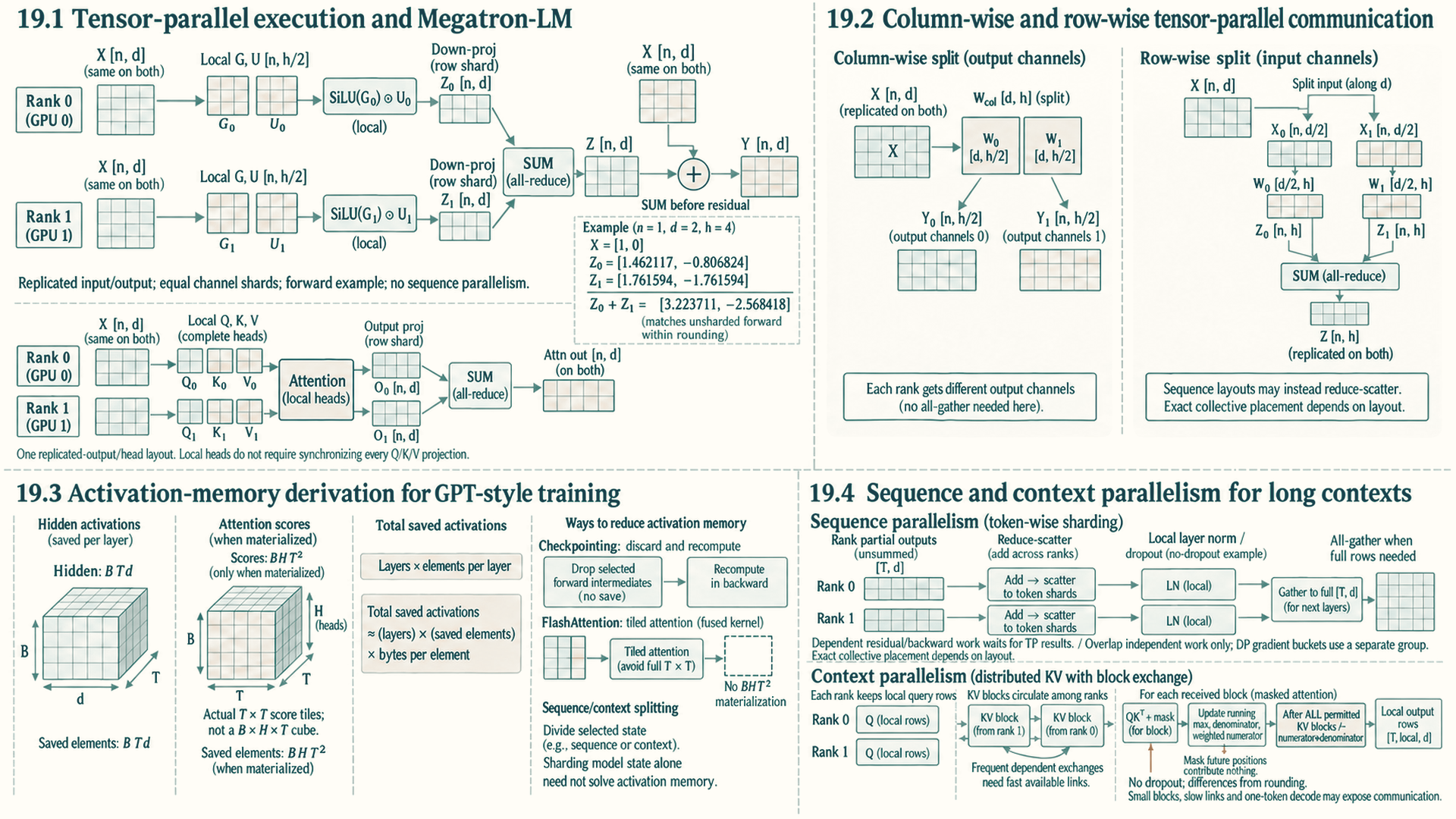
Tensor, sequence, and context parallelism divide different objects within a model execution. Pipeline stages and expert placement follow in the next chapter. Their memory savings and communication schedules are therefore different. A usable layout identifies the local tensors, the result needed by the next operation, and the links carrying that result. The parallelism degree is the number of ranks in a group for one kind of parallel work. Combining strategies also requires checking the runtime’s group definitions. With one rank per GPU, those counts give the GPU total only when they describe independent ways of dividing the work.
19.1 Tensor-parallel execution and Megatron-LM
Model parallelism splits one model execution across ranks. Tensor parallelism divides work inside a layer, as in Megatron-LM: Training Multi-Billion Parameter Language Models Using Model Parallelism1. The partial result must reach the ranks that need it before the next dependent operation can run.
A column-parallel linear layer splits output channels across ranks. Each rank computes its output slice from the full input. A row-parallel linear layer splits input channels across ranks. Each rank computes a partial output, and those partial outputs must be summed.
The forward layouts below start and end with replicated hidden states, use equal channel shards and complete local attention heads, and do not use sequence parallelism (Section 19.4). Backward has additional gradient dependencies, and other layouts can change the collective choice.
Two common forward-path partitions show where collective communication appears:
- MLP block sharding: In the three-matrix gated MLP counted in Section 10.4, matching columns of the gate and up projections belong to the same rank. That rank applies the activation and elementwise gate locally before its row-parallel down projection.
- Self-attention block sharding: The query, key, and value projections are sharded column-parallel, keeping attention head computations local to each GPU. The attention output projection is sharded row-parallel, requiring a single all-reduce before the residual connection.
The sigmoid linear unit (SiLU), also called Swish-1, applies \(\operatorname{SiLU}(a)=a/(1+e^{-a})\) to each scalar element.
In this layout, each rank computes matching gate and up channels and combines them element by element, so that intermediate stays local. Its down-projection shard produces a partial hidden vector. SUM all-reduce adds those partial vectors before the residual connection uses the complete result.
Example: A gated MLP across two ranks
The goal is to reproduce a full MLP forward output while dividing its intermediate channels. This example uses a bias-free SwiGLU feed-forward layer, a gated MLP whose Swish-1 activation and three-matrix operation are defined in GLU Variants Improve Transformer.2 The partition below applies the column/row split to that operation. It is a forward-only mathematical trace, not a complete training program or a claim that the original Megatron-LM paper used SwiGLU.
Both ranks receive the same \(X\) of shape \([n,d]\), with \(n\) token rows and \(d\) hidden features. Let \(h\) be an even intermediate width and \(i\) be rank 0 or 1. Each rank holds gate and up matrices \(W_{g,i}\) and \(W_{u,i}\), each shaped \([d,h/2]\), with matching intermediate-channel indices. Its down-projection shard \(V_i\) has shape \([h/2,d]\).
The local projections are \(G_i=XW_{g,i}\) and \(U_i=XW_{u,i}\), both shaped \([n,h/2]\). The gated intermediate is \(Y_i=\operatorname{SiLU}(G_i)\odot U_i\), where \(\odot\) multiplies matching elements, so \(Y_i\) also has shape \([n,h/2]\). Each rank then computes \(Z_i=Y_iV_i\) of shape \([n,d]\). SUM all-reduce returns \(Z=Z_0+Z_1\) with shape \([n,d]\) on both ranks. Because the gate acts independently on matching local channels, no intermediate gather is needed for this layout.
For a numerical trace, let \(n=1\), \(d=2\), \(h=4\), and \(X=[1,0]\). These small dimensions illustrate the operation, not a production expansion ratio. The matrices below list rows in brackets:
| Rank | Gate matrix | Up matrix | Down matrix |
|---|---|---|---|
| 0 | \([[1,-1],[0,0]]\) | \([[2,3],[0,0]]\) | \([[1,0],[0,1]]\) |
| 1 | \([[0,2],[0,0]]\) | \([[4,1],[0,0]]\) | \([[1,1],[1,-1]]\) |
Rank 0 obtains \(G_0=[1,-1]\) and \(U_0=[2,3]\). Applying SiLU gives approximately \([0.731059,-0.268941]\), so \(Y_0=[1.462117,-0.806824]\) and \(Z_0=Y_0\). Rank 1 obtains \(G_1=[0,2]\) and \(U_1=[4,1]\), giving \(Y_1=[0,1.761594]\) and \(Z_1=[1.761594,-1.761594]\). The all-reduce returns approximately \(Z=[3.223711,-2.568418]\) to each rank. The unsharded calculation concatenates the gate/up columns and stacks the down-matrix rows, producing the same sum apart from floating-point rounding.
Conclusion: The gate is a nonlinear, elementwise step between projections. Its output can stay local because both branches use the same channel partition. The down projection produces partial hidden vectors that must be added before the residual path uses them.
The key performance fact is where the collective is placed. Tensor parallelism tries to keep intermediate slices local through several operations, then synchronizes only when the full hidden vector is needed by the residual path, normalization, or the next block.
| Transformer subpath | Local tensor-parallel work | Collective placement | Why the placement matters |
|---|---|---|---|
| MLP gate/up projection | Matching column shards produce local G and U, then Y = SiLU(G) times U elementwise | No immediate forward all-reduce | Activation and gating stay local because both branches use matching channels |
| MLP down projection | Row-parallel input channels; each rank computes a partial hidden output | All-reduce after the down projection | Partial sums must be combined before the residual connection |
| Attention Q/K/V projection | Complete attention heads are assigned to ranks in this layout | Often no immediate all-reduce | Attention for local heads can proceed without synchronizing every projection |
| Attention output projection | Each rank computes a partial contribution back to hidden dimension | All-reduce before block output is complete | The next residual or layer needs the full hidden vector |
19.2 Column-wise and row-wise tensor-parallel communication
Column-wise and row-wise tensor parallelism describe where a linear layer is split and where the ranks must communicate. The distinction matters because splitting output channels and splitting input channels place collective operations at different points in the transformer block.
Megatron-LM-style tensor parallelism chooses where communication occurs by pairing column-parallel and row-parallel projections inside transformer blocks, following Megatron-LM: Training Multi-Billion Parameter Language Models Using Model Parallelism3. With the column-parallel split introduced in Section 19.1, each rank computes its own output slice from the full input, so the forward pass can avoid an immediate all-reduce. The backward pass accumulates gradients for each local weight shard and may need to combine input gradients depending on how the following layer is arranged. Exact collectives depend on the layer and sequence-parallel configuration.
For the row-parallel split introduced in Section 19.1, partial outputs from the ranks must be summed. In the replicated-output layout used above, that summation is an all-reduce in the forward path. Sequence-parallel layouts can instead reduce-scatter the output. The need to communicate inside each layer is why tensor parallelism is usually kept inside fast NVLink or NVSwitch domains.
The placement intuition is: keep attention heads or MLP intermediate channels local as long as possible, then reduce only when the full hidden vector is needed by a residual connection, normalization, or the next block boundary. This reduces communication frequency compared with naively synchronizing after every projection.
In the forward MLP trace in Section 19.1, the residual computation waits for the tensor-parallel sum. Backward likewise must combine partial input gradients before dependent earlier work uses them. Overlap is possible only with computation that does not need the pending result and with a schedule that permits both operations to run. If training also uses data parallelism, a separate group synchronizes corresponding parameter-shard replicas with gradient buckets. Those buckets serve the data-parallel group and do not remove the tensor-parallel layer dependencies.45
Compared with DDP gradient buckets, layer-internal collectives often have little independent work after them. Their exposed delay can be harder to hide when the next layer needs the result.
19.3 Activation-memory derivation for GPT-style training
Large-model training often hits the activation wall before the parameter wall. Parameters are static with respect to batch size and sequence length, but saved activations grow with both. In GPT-style transformers, attention score tensors can also scale quadratically with sequence length if the implementation materializes them.
Saved activation storage follows from two common tensor shapes. Let \(B\) be local micro-batch size, \(T\) sequence length, \(d\) hidden width, \(H\) attention-head count, \(L\) local transformer layers, and \(b\) bytes per stored element.
- A hidden-sized tensor has \(BTd\) elements and occupies \(BTdb\) bytes per layer.
- A materialized dense attention matrix has \(BHT^2\) elements and occupies \(BHT^2b\) bytes per layer.
If each layer saves \(n_{\text{hidden}}\) hidden-sized tensors and \(n_{\text{score}}\) attention-matrix-sized tensors, their combined payload is approximately
\[ A \approx Lb\left(n_{\text{hidden}}BTd+n_{\text{score}}BHT^2\right). \]
For an illustrative calculation, assume \(n_{\text{hidden}}=16\), \(n_{\text{score}}=1\), \(B=1\), \(T=2048\), \(d=4096\), \(H=32\), \(L=10\), and \(b=2\) bytes. This uses the same coarse hidden-tensor count as Chapter 9 so the two estimates can be compared.
\[ A \approx 10\cdot2\left(16\cdot2048\cdot4096+32\cdot2048^2\right) =5{,}368{,}709{,}120\ \text{bytes}=5\ \text{GiB}. \]
These are assumed tensor counts, not measurements of a particular model. Actual counts depend on the layer implementation, backward algorithm, recomputation policy, and fused kernels. The estimate excludes weights, gradients, optimizer state, temporary workspaces, and allocator overhead. Measure peak allocation before using it as a device-memory budget.
Several techniques change the saved tensors. Activation checkpointing discards selected forward intermediates and recomputes them during backward. FlashAttention-style kernels avoid materializing the full attention matrix. Sequence and context parallelism divide the sequence dimension across GPUs (Section 19.4). The exact per-rank saving depends on which tensors each implementation keeps or reconstructs.
This derivation explains why FSDP or tensor parallelism alone can leave training memory limited by activations. FSDP shards model state, while activations remain tied to local micro-batch and layer execution unless activation checkpointing, sequence parallelism, FlashAttention, or smaller micro-batches reduce them.
19.4 Sequence and context parallelism for long contexts
Tensor parallelism divides the weights of a layer, but every tensor-parallel rank still holds activations for the whole sequence in the operations it does not split, and attention state grows with the sequence. At long context lengths, that per-GPU state becomes the limit. Two methods divide the sequence dimension itself.
- Sequence parallelism splits the sequence across the tensor-parallel ranks for the operations that tensor parallelism leaves replicated, such as layer normalization and dropout. Where the following operation can run on separate token-row shards, reduce-scatter adds the partial outputs while leaving each rank with only its assigned rows. All-gather later restores the full row collection when another operation needs it. In the earlier replicated-output MLP, by contrast, all-reduce leaves the full sum on both ranks before the residual path. The exact collective positions depend on the layout; they do not follow from every row-parallel layer. Together with selective recomputation, Korthikanti et al. report a 5 times reduction in activation memory while almost eliminating the need to recompute activations.6
- Context parallelism splits the sequence through attention as well. In a simple block partition, each rank holds one block of the sequence’s queries, keys, and values. Ring Attention circulates key and value blocks and can overlap their transfer with attention on a block already present. Its blockwise method preserves the attention operation, apart from floating-point rounding, and can scale the supported sequence length with device count. Full overlap requires enough computation per block relative to communication time.7
For the no-dropout attention calculation in Section 5.7, each rank keeps its query rows and updates their running maximum, denominator and value-weighted numerator as KV blocks arrive. Masked positions contribute nothing. After all permitted keys have contributed, dividing the accumulated numerator by the denominator gives that rank’s output rows.8
Splitting the stored keys and values across GPUs does not by itself reduce all training memory per GPU by the same factor. The following estimate uses a training/prefill-sized query block, not a one-token decode step. A profile must include startup, temporary buffers, rank imbalance, and the actual attention schedule. Small blocks, slow links, and one-token decode can expose communication even when a long-block estimate looks favorable. A fast scale-up domain reduces that risk (Section 17.4).
Example: A 128k-token sequence on eight GPUs
Inputs: A full-sequence forward attention pass with Llama 3 8B-like shapes (32 layers, 32 query heads, 8 KV heads, \(d_h=128\), BF16), one sequence of 131,072 tokens, and context parallelism over 8 GPUs, so each holds a block of 16,384 tokens. The link rate of 400 GB/s and compute rate of 989 TFLOP/s are illustrative inputs to the estimate, not measurements.
Memory: Storing keys and values for the full sequence across all 32 layers requires 16 GiB with these shapes (Section 12.7). Partitioning that payload evenly gives 2 GiB per GPU. This counts the resident KV shards only, not queries, outputs, received KV buffers, backward state, or other saved activations. In training, these tensors are activations rather than a persistent decode cache.
Overlap: In one layer, one KV block is \(2\times16{,}384\times8\times128\times2\approx67\) MB, which takes about 0.17 ms at the assumed 400 GB/s, excluding startup and contention. Dense attention from a 16,384-token query block to one 16,384-token KV block takes \(4\times16{,}384^2\times32\times128\approx4.4\times10^{12}\) FLOPs, about 4.4 ms at the assumed 989 TFLOP/s. For contiguous causal blocks, an earlier KV block contributes a full block of attention, the diagonal block contributes roughly half, and a future block is fully masked. Useful compute and rank balance therefore depend on block order and the causal schedule.
Conclusion: For a block pair with substantial attention work, this estimate leaves room to hide the next transfer behind computation. It does not establish full overlap for the complete causal pass or divide all training memory by eight.
Tensor-parallel groups should remain on the fastest available links when each layer requires frequent communication.
References
Shoeybi, M., Patwary, M., Puri, R., LeGresley, P., Casper, J., & Catanzaro, B. (2019). Megatron-LM: Training Multi-Billion Parameter Language Models Using Model Parallelism. Preprint at Megatron-LM paper (DOI), v1 submitted 2019-09-17, v4 revised 2020-03-13. Supports intra-layer model parallelism with column-parallel and row-parallel linear layers separated by a small number of collectives, orthogonal to pipeline parallelism. Limit: exact collective placement depends on layer and sequence-parallel configuration; reported PetaFLOP and scaling efficiency apply to tested 8.3 billion parameter setups on 512 GPUs.↩︎
Shazeer, N. (2020). GLU Variants Improve Transformer. arXiv:2002.05202v1, Section 2, equations 5-6. GLU Variants Improve Transformer. Supports the bias-free three-matrix SwiGLU operation with a Swish-1 gate. The two-rank partition and numerical values are a teaching derivation of that operation, not performance results from the paper. This is the same work cited for sizing in the inference chapter.↩︎
Shoeybi, M., Patwary, M., Puri, R., LeGresley, P., Casper, J., & Catanzaro, B. (2019). Megatron-LM: Training Multi-Billion Parameter Language Models Using Model Parallelism. Preprint at Megatron-LM paper (DOI), v1 submitted 2019-09-17, v4 revised 2020-03-13. Supports intra-layer model parallelism with column-parallel and row-parallel linear layers separated by a small number of collectives, orthogonal to pipeline parallelism. Limit: exact collective placement depends on layer and sequence-parallel configuration; reported PetaFLOP and scaling efficiency apply to tested 8.3 billion parameter setups on 512 GPUs.↩︎
Shoeybi, M., Patwary, M., Puri, R., LeGresley, P., Casper, J., & Catanzaro, B. (2019). Megatron-LM: Training Multi-Billion Parameter Language Models Using Model Parallelism. Preprint at Megatron-LM paper (DOI), v1 submitted 2019-09-17, v4 revised 2020-03-13. Supports intra-layer model parallelism with column-parallel and row-parallel linear layers separated by a small number of collectives, orthogonal to pipeline parallelism. Limit: exact collective placement depends on layer and sequence-parallel configuration; reported PetaFLOP and scaling efficiency apply to tested 8.3 billion parameter setups on 512 GPUs.↩︎
PyTorch. (2026). Distributed Data Parallel. Versioned v2.14 design note at Distributed Data Parallel design note, created 2026-05-16 and updated 2026-05-16, describing implementation state as of v1.4. Supports Reducer gradient buckets with
bucket_cap_mb, autograd hooks, per-bucket async all-reduce with mean gradients, same-order all-reduce across ranks, and overlap of collectives with backward compute. Limit: input sharding is done by the application, for example with a distributed sampler; DDP synchronizes gradients but does not partition inputs by itself.↩︎Korthikanti, V., Casper, J., Lym, S., McAfee, L., Andersch, M., Shoeybi, M., & Catanzaro, B. (2022). Reducing Activation Recomputation in Large Transformer Models. arXiv:2205.05198. Supports sequence parallelism and selective activation recomputation used with tensor parallelism, reducing activation memory by 5x and almost eliminating recomputation in the paper’s models up to one trillion parameters. Limit: the savings depend on the model and the recomputation policy.↩︎
Liu, H., Zaharia, M., & Abbeel, P. (2023). Ring Attention with Blockwise Transformers for Near-Infinite Context. arXiv:2310.01889. Supports distributing long sequences across devices with blockwise attention and feed-forward computation, fully overlapping key-value block communication with computation, and sequences up to device count times longer without approximation. Limit: full overlap requires enough computation per block relative to link speed.↩︎
Liu, H., Zaharia, M., & Abbeel, P. (2023). Ring Attention with Blockwise Transformers for Near-Infinite Context. arXiv:2310.01889. Supports distributing long sequences across devices with blockwise attention and feed-forward computation, fully overlapping key-value block communication with computation, and sequences up to device count times longer without approximation. Limit: full overlap requires enough computation per block relative to link speed.↩︎