2 Workload phases and live memory
Training and serving run related model operations, but they keep different tensors (multidimensional arrays of numbers) in memory and move different bytes during each phase. Explaining their performance starts with the different results they produce.
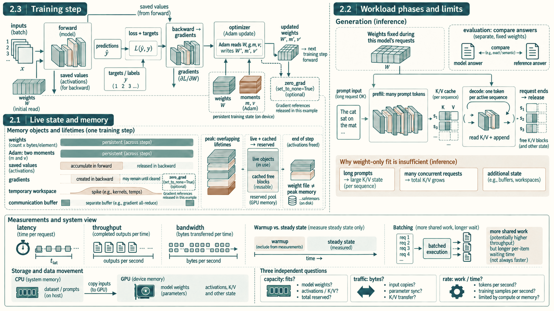
During training, the model receives examples and predicts outputs. A loss (a single number measuring how wrong the predictions are) compares those predictions with target answers, backward propagation computes how the loss depends on the weights (the model’s learned numbers, also called parameters), and an optimizer (the update rule) changes those weights. During text generation, the weights stay fixed: the model processes a prompt, produces scores for the next token (one unit from the tokenizer vocabulary), and a selection rule chooses that token. Repeating this step extends the output. The initial prompt processing is called prefill, and the repeated one-token steps are decode. Retained attention state (Section 2.1), called the key-value (KV) cache, lets later steps reuse earlier work. Evaluation also keeps weights fixed, but compares predictions with reference answers to measure quality.
The same tensor properties appear in two distinct execution regimes. Training changes parameters and retains backward state. Inference serving keeps parameters fixed while maintaining request and cache state. The comparison below names the goal, live objects, phases, and measurements for each regime.
- Training: Repeated execution that updates model parameters from data.
- Goal: Improve the objective while maximizing useful tokens per second, numerical stability, and hardware utilization.
- Live objects: Parameters, activations, gradients, optimizer state, temporary workspaces, and often communication buffers (all defined in the next section).
- Phases: Forward propagation, loss computation, backward propagation, optimizer step, and distributed synchronization when several cooperating processes are used. Each process has a rank (its integer identity within the distributed group, Section 3.4); usually one process runs per GPU.
- Measurements: Training tokens per second, step time, time to target quality, memory headroom, scaling efficiency, and numerical stability.
- Inference serving: Repeated requests that use fixed model weights to produce outputs.
- Goal: Meet latency, throughput, quality, and cost targets under a service workload.
- Live objects: Parameters, temporary activations, KV cache, scheduler metadata, request queues, sampling state (the selection rule’s settings and random state), and sometimes communication buffers.
- Phases: Tokenization, request admission, prefill, decode, post-processing, and streaming.
- Measurements: Serving measurements describe waiting, streaming speed, and completed work. Chapter 10 develops these quantities and their measurement boundaries.
2.1 Live state and memory
The preceding chapter defined the individual objects. Backward propagation sometimes needs values from forward. For example, let \(y=wx\) and let a scalar loss \(J\) depend on \(w\) only through \(y\). The chain rule gives \(\partial J/\partial w=(\partial J/\partial y)x\): computing the parameter gradient needs the forward input \(x\). PyTorch retains the values required by the recorded backward rules until those rules have used them. This does not mean every intermediate value is saved.
Memory pressure depends on which objects overlap in time. Parameters and optimizer buffers may stay live for the whole training step. Saved activations accumulate during forward. Gradients appear during backward. Temporary workspaces can raise the peak even though they exist briefly. In serving, model weights remain fixed while admitted requests grow and release KV-cache blocks.
A profiler (a tool that records where time and memory go) can measure time and byte traffic for a selected phase. Allocator memory statistics report allocated and reserved capacity; achieved bandwidth requires bytes and elapsed time measured over the same phase.
Parameters: Learned weights. They are used in both training and inference. Footprint scales with parameter count and dtype. For example, a 7B-parameter model in FP16 or BF16 is roughly 14 GB before metadata, fragmentation, and engine overhead.
Gradients: Derivatives of the loss with respect to parameters. Backward propagation computes them; the optimizer reads them to calculate an update. Their tensors can remain live between backward and the update.
Activations: Intermediate tensors produced by forward propagation. Training often saves them for backward propagation. Inference usually releases most of them quickly. Footprint scales with batch size, sequence length, hidden dimension, layer count, precision, and checkpointing policy.
Optimizer state: Extra buffers used by optimizers such as Adam or AdamW (update rules that keep running averages of each gradient and its square). Adam-style first and second moments can exceed the parameter footprint when stored in FP32, which is why optimizer state becomes a training memory wall. Adam maintains biased first and second moment estimates as described in Adam: A Method for Stochastic Optimization1, and ZeRO partitions optimizer states, gradients, and parameters across data-parallel ranks as described in ZeRO: Memory Optimizations Toward Training Trillion Parameter Models2.
Temporary workspaces: Short-lived buffers allocated by kernels, vendor libraries, compilers, or serving engines. They affect peak memory and can cause out-of-memory failures.
Key-value (KV) cache: Inference-serving attention state that stores previous keys and values so decode does not recompute the full prefix.
Communication buffers: Intermediate tensors used for a collective operation (a communication step in which every participating rank takes part), such as all-reduce (combining the ranks’ tensors, for example by elementwise summation, and giving the result to every rank), all-gather, reduce-scatter, and all-to-all (Section 16.2), or for point-to-point transfers. They appear in distributed training and distributed inference and can create memory spikes as well as network traffic.
A model that fits in one mode may fail in another. A model checkpoint (the saved weights file) that fits for inference may not fit for training once gradients and optimizer state are added. A model that fits short prompts may fail under long-context serving because KV cache grows with admitted requests and sequence length.
Peak-memory lifecycle
Before forward: Parameters, input tensors, and persistent buffers are live. Optimizer state is also live after initialization, although some optimizers allocate their buffers lazily at the first update. The model may appear to fit at this point while the upcoming step still cannot run. During forward: Each layer produces activations. Training keeps many of them alive because backward propagation uses the original values. Inference usually releases most temporary activations quickly. At loss and backward start: The loss is the starting point for backward traversal of the autograd graph. Backward reads saved activations, writes gradients, and may allocate temporary workspaces for backward kernels.
During the optimizer update: The optimizer reads parameters, gradients and its state, then writes updated parameters and state. Parameter and gradient tensors, optimizer buffers and any update workspaces contribute to this phase’s live memory. Lazily initialized optimizer buffers can raise the peak when they are first allocated.
After a training step: Backward normally releases saved activations as it consumes them. Gradients may be set to None after the update; a retained autograd graph or other references can keep some tensors live. Allocator-reserved memory can remain high because the PyTorch caching allocator keeps freed GPU memory blocks for reuse instead of returning them (Section 4.3).
Live memory includes weights, activations, temporary workspaces and, during serving, KV-cache blocks. The allocator’s reserved pool includes the live allocations it manages plus blocks retained for reuse; reserved and live bytes are not separate amounts to add. Whether the next allocation fits also depends on free device memory and whether a suitable block is available. Checkpoint size alone does not describe that state.
2.2 Workload phases and limits
Diagnosing a phase requires fixed meanings for the words used to describe speed, because “fast” can refer to one request, a whole service, or one piece of hardware. The rest of the guide uses these meanings:
- Latency: elapsed time for one piece of work, from its start to its completion, such as one training step or one request.
- Throughput: completed work per unit of time across many pieces of work, such as tokens per second or requests per second. Processing work in larger batches often raises throughput while raising each item’s latency.
- Bandwidth: the rate at which a memory or link can move bytes. An H100 SXM GPU’s HBM is specified at 3.35 TB/s (Section 3.6). Achieved bandwidth is the measured bytes divided by the measured time.
- Utilization: the fraction of a resource’s capacity, or of the time, that is in use. A utilization figure is meaningful only with its resource and definition. The “GPU utilization” reported by monitoring tools is a narrow time measure (Section 6.3).
- Saturation: a resource running at its limit, so that additional demand waits in a queue instead of being served faster.
- Critical path: the longest chain of dependent work in a step. For a modeled execution whose dependencies include required serialization and resource waits, this chain sets completion time. A graph of data dependencies alone gives a lower bound when limited resources can add waiting. Shortening it helps until another required chain becomes limiting. If several longest chains tie, shortening only one may leave completion time unchanged. Overlapping work is hidden only when it neither extends the required chain nor slows it by competing for resources.
- Steady state: repeated execution after one-time setup, such as compilation, memory allocation, and cache filling, has finished. Measurements in this guide refer to steady state unless they say otherwise.
Check footprint by asking whether the live objects fit. Check traffic by asking how many bytes the phase reads and writes. Check throughput by asking how quickly the hardware can perform those transfers or calculations. Diagnose a phase by measuring these separately. Fitting in HBM does not show that HBM bandwidth is sufficient.
- Bandwidth and locality: The rate and distance at which bytes must reach the computation. Reuse in on-chip storage (registers, shared memory, or cache, Section 3.2) reduces traffic to slower memory tiers.
- Compute throughput: The rate of useful arithmetic work for the phase, interpreted together with tensor shapes, precision, and hardware utilization.
- Launch and control overhead: Time spent in Python dispatch, framework dispatch, kernel launches, compiler transitions, or scheduler decisions.
- Communication and synchronization: Time spent moving tensors across GPUs or ranks and waiting for participants to reach compatible execution points.
Diagnose one phase at a time by naming the work, the live objects, the target measurement, and the resource whose capacity, throughput, or dependency is exhausted.
Performance-change key: Do less work removes operations that do not change the required result. Move fewer bytes reuses data closer to computation. Use the hardware better gives arithmetic units enough suitable work. Wait or launch less shortens host gaps and avoidable dependencies. Keep less state live reduces the memory needed at one time. Share work across devices adds capacity or throughput but also adds communication. These are possible effects, not a diagnosis: measure the phase first, then use the later hardware and software chapters to test which change actually helps.
- Training forward: Reads parameters and input batches, writes activations, and often uses large matrix operations that run on Tensor Cores (the GPU’s dedicated matrix-multiply units, Section 3.3). Likely bottlenecks are compute throughput, activation memory, and HBM traffic. See the complete training update and operation counts.
- Training backward: Reads saved activations and parameters, writes gradients, and may recompute activations when activation checkpointing is used. Likely bottlenecks are activation memory, HBM bandwidth, and gradient computation. See saved activations and gradient accumulation.
- Optimizer step: Reads parameters, gradients, and optimizer state, then writes updated parameters and state. Likely bottlenecks are memory bandwidth and optimizer-state footprint. See training state and precision and sharded updates.
- Prefill: Processes prompt tokens and builds initial KV cache. It often forms large matrix operations over many tokens and can be compute-heavy. Likely bottlenecks are compute throughput, temporary activation and workspace memory, and attention traffic for long prompts. See request phases, the decode loop and its cache, and request scheduling.
- Decode: Generates one token at a time while reading parameters and the existing KV cache, then appending new KV entries. Likely bottlenecks are HBM bandwidth, launch overhead, batching, and cache layout. See request phases, the decode loop, and request scheduling.
- Distributed synchronization: Moves gradients, parameters, activations, routed token representations for mixture-of-experts layers (Section 20.2), or partial layer results between ranks. Likely bottlenecks are interconnect bandwidth, latency, topology, rank skew (ranks reaching a shared step at different times), and collective scheduling. See collective results, distributed measurements, and the later training layouts.
2.3 Training step
Section 2.2 identified the measurements and resource limits that can change across workload phases. A supervised training loop makes those phases concrete. Each repeated step moves input data to the GPU, runs forward computation to produce predictions, compares predictions with labels through the loss function, computes gradients through backward propagation, updates parameters through the optimizer, and may synchronize distributed workers. Later chapters improve these same moments through placement, kernels, precision, graph capture (compiler capture records tensor operations for optimization, whereas CUDA Graph recording records GPU work for replay, Chapter 8), sharding, and communication scheduling.
- Forward propagation: Reads inputs and parameters, writes outputs, and may save activations for backward propagation.
- Loss computation: Turns predictions and labels into the scalar or batched objective being optimized.
- Backward propagation: Traverses the recorded computation in reverse to produce gradients.
- Optimizer step: Updates parameters using gradients and optimizer state.
- Device placement: Determines whether tensors live on CPU memory, GPU HBM, or another device, and therefore which transfers and execution paths the step uses.
The loop also explains why memory and timing need separate measurements. Forward computation saves activations for backward; backward consumes them and writes gradients; the optimizer reads parameters, gradients, and its own state, then writes updated parameters and state. Memory peaks where these objects overlap in time, while elapsed time depends on the computation and transfers that cannot overlap.
References
Kingma, D. P., & Ba, J. (2015). Adam: A Method for Stochastic Optimization. 3rd International Conference on Learning Representations. Adam paper on arXiv (v1 2014-12-22; v9 2017-01-30). Support: Adam uses adaptive first-order moment estimates. Limit: the guide’s FP32 footprint comparison is an applied sizing consequence, not a quoted source result.↩︎
Rajbhandari, S., Rasley, J., Ruwase, O., & He, Y. (2020). ZeRO: Memory Optimizations Toward Training Trillion Parameter Models. ZeRO paper on arXiv (v3 2020-05-13). Support: ZeRO partitions optimizer states (Stage 1), gradients (Stage 2), and parameters (Stage 3) across data-parallel ranks. Section 3.1 counts mixed-precision Adam as 2 bytes of fp16 parameters, 2 bytes of gradients, and K = 12 bytes of fp32 parameter copy, momentum, and variance, 16 bytes per parameter in total. Limit: FSDP details and the guide’s sharding tradeoffs are separate framework behavior covered in later chapters.↩︎