1 Model operations and tensors
1.1 The model behind the workload
Producing text can be slow, and learning from examples can require more memory than using the resulting model. Explaining either cost starts with the computation and the numerical state it uses.
A model is a computation with learned numerical values, called weights or parameters. A language model takes text as input and computes scores used to choose a continuation. A forward pass applies the model to an input to produce predictions. During inference, those parameters stay fixed while the model produces an output.
During training, a loss measures disagreement between predictions and target answers and supplies the starting value for backward propagation. Backward propagation computes gradients, derivatives of that loss with respect to the parameters. An optimizer uses the gradients to update the parameters. During evaluation, predictions are compared with held-out reference answers to measure quality, without updating parameters. Transfers, communication, and serving controls support these operations. Locating a slow operation or a large stored object requires a picture of the computation, its supporting work, and their sizes before considering the hardware.
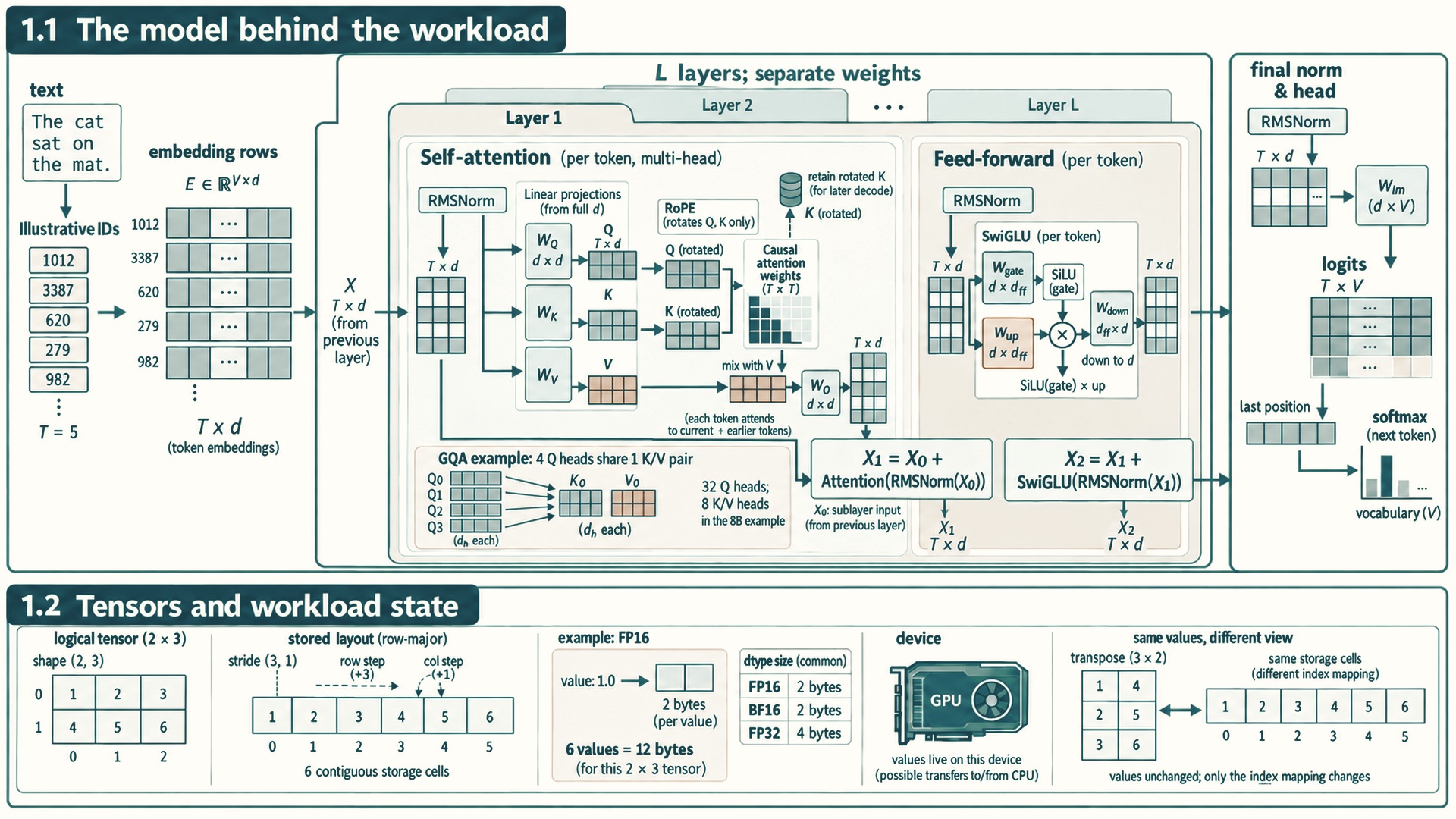
Text first becomes numbers. A tokenizer maps text to a sequence of token units from its vocabulary, the fixed collection it represents. A token can be a word, part of a word, punctuation, whitespace, a byte sequence, or a special control marker. Each unit is represented by an integer token ID, its position in that vocabulary. A language-model forward pass turns the sequence into scores for the next token. Llama 3 uses a vocabulary of about 128,000 tokens.1 Section 10.1 treats tokenizers and why the token count drives cost. From there, a Llama-style decoder-only language model applies the four stages below. Other model families can use different normalization and feed-forward choices.
- Embedding: Each token ID selects one row of an embedding table (a matrix holding one learned vector per vocabulary entry). The vector has \(d\) numbers, the hidden width or model dimension. A sequence of \(T\) tokens therefore becomes a \(T\times d\) matrix, the hidden state.
- Layers: The hidden state passes through \(L\) structurally similar layers, also called transformer blocks, with separately learned weights. Each layer has two sub-layers, and each sub-layer follows the same pattern: normalize its input, transform it, and add the result back to the input.
A projection is a learned matrix operation. Three projections form queries, keys, and values. Attention compares queries with keys and mixes values from the current and earlier token positions, with no separate learned weights for that comparison and mixing. A fourth projection returns the mixed result to width
d. The feed-forward multilayer perceptron (MLP) transforms each token independently using projections and a nonlinear function. In the Llama-style SwiGLU form, gate and up projections each expand hidden widthdto intermediate widthd_ff. The nonlinear gate result is multiplied element by element by the up result, then returned todby the down projection. RMSNorm divides each token's vector by its root-mean-square magnitude, with a small stabilizing term, then applies learned per-feature scaling. Residual connections add each sub-layer's output to its input.Inside a transformer layer: attention, feed-forward computation, and residual connections- The attention sub-layer is the part of a layer that combines information across permitted token positions. In this model, it first applies RMSNorm: it divides each token’s vector by its root-mean-square magnitude, with a small stabilizing term, then applies learned per-feature scaling. Three projections (multiplications by learned weight matrices) then produce a query, a key, and a value vector for every token. Llama applies rotary position embedding (RoPE), a position-dependent rotation of queries and keys, before comparing them. Their comparison then depends on the tokens’ relative positions.2 The rotated keys are retained for later decode steps. Attention compares each token’s query with the keys of the permitted positions and mixes the matching values. In a causal language model, a token may use only itself and earlier positions. The projected vectors are split into attention heads, separate attention calculations using head-sized query, key, and value vectors. Each projection reads the whole input vector, rather than just one slice of its features. Each head’s vectors have length \(d_h\), the head dimension. An output projection maps the result back to width \(d\). Section 5.6 works through the attention arithmetic.
- The feed-forward sub-layer is the part that transforms each token’s vector independently, using the same learned matrices at every position. It applies another RMSNorm and then a multilayer perceptron (MLP) (a pair of large projections with a nonlinear function between them). Llama-style models use the SwiGLU form, which has three weight matrices.3 Its gate and up projections each map the token’s vector from width \(d\) to \(d_{ff}\). A nonlinear function transforms the gate result, which then multiplies the up result element by element. The down projection maps this combined \(d_{ff}\) vector back to width \(d\).
- A residual connection (adding a sub-layer’s output to its input) follows each sub-layer, so the hidden state keeps its \(T\times d\) shape from layer to layer.
- Output: A final RMSNorm and the language-model head (a \(d\times V\) projection, where \(V\) is the vocabulary size) turn the hidden state into logits: one unnormalized score per vocabulary entry for each position.
- Selection: A decoding rule turns the last position’s logits into the next token, as described at the end of this section.
Most parameters, about 87 percent in the 8B example below, sit in stage 2’s learned matrices. Attention and MLP gate/up projections consume a \(T\times d\) state. The MLP down projection consumes the \(T\times d_{ff}\) intermediate and returns \(T\times d\). These matrix multiplications are the operations that GPU hardware (Chapter 3) and GPU libraries (Chapter 4) are built to accelerate. The query, key, value, and output projections have learned weights. Comparing queries with keys and using the resulting scores to combine values adds no separate learned matrix, but this work grows with sequence length. Decode also retains keys and values, which is why the KV cache receives separate treatment in Section 2.1 and Chapter 10 and Chapter 12.
The final stage chooses one token from the logits. Softmax (exponentiating each score and dividing by the sum, so the scores become probabilities, Section 5.6) converts logits into a probability distribution over the vocabulary. A decoding rule then selects from it:4
Greedy decoding takes the highest-probability token. Temperature changes how concentrated the probabilities are. Top-k and top-p restrict which tokens can be sampled. Beam search tracks several continuations. Random sampling can change repeated outputs, and even greedy results can change when floating-point rounding flips a close choice.
- Greedy decoding picks the most probable token. It is deterministic in principle: the same prompt and the same arithmetic give the same output, although changes in batching or kernel choice can alter floating-point rounding enough to flip a close choice.
- Temperature uses \(t>0\) to divide the logits before softmax. Values between 0 and 1 concentrate probability on likely tokens, and values above 1 spread it out. The formula requires positive temperature; greedy decoding is the separate highest-probability rule above, not evaluation of the formula at zero.
- Top-k sampling draws from only the \(k\) most probable tokens, using their probabilities renormalized to sum to one.
- Top-p (nucleus) sampling orders tokens from highest to lowest probability, keeps the shortest prefix whose probabilities add up to at least \(p\) for \(0<p\leq1\), and samples after renormalizing that prefix.
- Beam search keeps several candidate continuations at once and extends the most probable ones, so it runs several sequences per request.
At each decode step, greedy or sampling selection chooses one next token per active sequence; beam search instead keeps several candidate continuations for one request. Selection is small next to the layers, but it can require sorting vocabulary scores or a round trip to the CPU. Random sampling can make repeated runs differ unless its random state and arithmetic are controlled. The scheduling chapter returns to its serving cost, and the comparison method to its effect on correctness checks.
The number of parameters in a projection is its input width times its output width. For a layer, the total adds the four attention projections, the three SwiGLU projections, and the normalization weights. Multiplying that layer total by \(L\) and adding the embedding and output matrices and final normalization weights gives the model total. Sharing a key and value head among several query heads is grouped-query attention: it narrows the key and value projections without reducing the number of query heads (Section 2.1).
Example: Where the parameters of an 8B model sit
Inputs: The published Llama 3 8B configuration has \(L=32\) layers, \(d=4{,}096\), 32 query heads and 8 key-value heads with \(d_h=128\), an MLP width \(d_{ff}=14{,}336\), and a vocabulary of about 128,000 tokens.5 Sharing each key and value head among four query heads means that the key and value projections produce \(8\times128=1{,}024\) numbers per token instead of 4,096.
| Weight matrix in one layer | Shape | Parameters |
|---|---|---|
| Query projection | \(4{,}096\times4{,}096\) | 16,777,216 |
| Key projection | \(4{,}096\times1{,}024\) | 4,194,304 |
| Value projection | \(4{,}096\times1{,}024\) | 4,194,304 |
| Attention output projection | \(4{,}096\times4{,}096\) | 16,777,216 |
| MLP gate and up projections (two matrices) | \(4{,}096\times14{,}336\) each | 117,440,512 |
| MLP down projection | \(14{,}336\times4{,}096\) | 58,720,256 |
| Two RMSNorm weight vectors | \(4{,}096\) each | 8,192 |
| Layer total | 218,112,000 |
Whole model: The 32 layers hold \(32\times218{,}112{,}000=6{,}979{,}584{,}000\) parameters. The embedding table and the language-model head each hold about \(128{,}000\times4{,}096=524{,}288{,}000\) when they are separate matrices. The total is about 8.03 billion, consistent with the model’s name. A tied design reuses the embedding matrix for the output projection and would reduce this illustrative total by about 0.52 billion parameters.
Conclusion: About 81 percent of each layer’s parameters sit in the MLP, and nearly all the rest in the four attention projections. Every generated token uses these dense projection matrices. Their stored size provides a first estimate of weight traffic for a small decode step when the weights exceed cache capacity and must be read from HBM. A batch can reuse each loaded weight across its token rows (Section 6.2).
The next section turns from these mathematical parts to the stored arrays that a measurement actually records.
1.2 Tensors and workload state
Section 1.1 named the model’s parts in mathematical terms. A performance measurement records the same parts as stored arrays: how many bytes each occupies, where it lives, and how its elements are laid out. Parameters, activations, gradients, logits, loss, and KV cache each carry a distinct storage and lifetime cost.
A tensor has a mathematical meaning and a physical storage description at the same time. Mathematically, it is a scalar, vector, matrix, or higher-dimensional array used in the model computation. Physically, it is a descriptor over storage: shape, dtype, strides, device, layout, storage offset, and sometimes gradient metadata. Performance depends on both descriptions. The PyTorch 2.4 documentation in Tensor Attributes describes dtype, device, layout, strided storage, and stride semantics used in this chapter.6
- Mathematical tensor: The array used in an operation, such as a vector of token embeddings, a matrix of weights, or a batch of logits.
- Tensor storage: The underlying bytes allocated on CPU memory, GPU High Bandwidth Memory (HBM) (a memory type used as main memory by GPUs such as H100, Section 3.2), pinned host memory (CPU memory locked in place so the GPU can copy it directly, Section 3.5), or another device-visible memory tier.
- Shape: The logical dimensions of the tensor. Shape controls matrix sizes, attention dimensions, batch sizes, and whether an operation can use an efficient kernel (a function that runs on the GPU, Section 3.1).
- Dtype: The numeric representation, such as FP32, BF16, FP16, FP8, INT8, or INT4 (32-bit, 16-bit, 8-bit, and 4-bit floating-point and integer formats, Section 9.4). Dtype controls bytes per element and can change which kernels are legal or fast.
- Device: Where the tensor lives, such as CPU memory or
cuda:0. Device placement controls which implementation PyTorch dispatches (selects and calls) and determines whether hidden transfers are needed. - Strides and layout: The mapping from logical indices to storage offsets. A stride gives the number of stored elements skipped when one index increases by one. For a contiguous row-major
2 x 3tensor with storage offset zero, strides(3, 1)place element(i, j)at offset3*i + jfrom its storage start: one row step skips three elements and one column step skips one. Contiguous here means that the logical row-major order occupies consecutive storage positions; a transpose can keep the same values while changing that mapping. - Autograd metadata: Training-time metadata used by PyTorch autograd (its automatic-differentiation engine) to know which operations produced a tensor and how to compute gradients.
This distinction explains several later performance issues. A transpose can be mathematically cheap while creating a non-contiguous view. A dtype change can halve memory traffic while selecting a different kernel path. A tensor’s device determines whether a copy is required. Autograd metadata can extend a tensor’s lifetime through backward propagation.
PyTorch is the Python framework used in the examples. torch.Tensor holds data and its shape, dtype, device, and stride metadata. torch.nn supplies model layers; torch.autograd records operations needed for gradients; torch.optim supplies parameter update rules. Later chapters introduce the measurement, compiler, and distributed interfaces when they are first used.
Example: Inspecting tensor identity
This example requires PyTorch and an available NVIDIA GPU usable through Compute Unified Device Architecture (CUDA), NVIDIA’s GPU programming platform (Chapter 4). For the contiguous 2 x 3 FP16 tensor below, expect shape (2, 3), dtype torch.float16, device cuda:0 or another selected CUDA device, stride (3, 1), True for contiguity, and 12 bytes of tensor payload. The device label can vary with the selected GPU.
import torch loads the PyTorch library. torch.randn(2, 3, ...) calls its tensor-creation function to make a random two-by-three tensor. device= and dtype= are Python keyword arguments: they pass values by parameter name. x.shape, x.dtype, and x.device read properties. Names followed by parentheses, such as x.stride(), call methods; numel() gives the element count and element_size() the bytes per element.
Code example: Inspecting tensor identity
import torch

x = torch.randn(2, 3, device="cuda", dtype=torch.float16)

print(x.shape)
print(x.dtype)
print(x.device)
print(x.stride())
print(x.is_contiguous())
print(x.numel() * x.element_size(), "bytes")
Conclusion: The trace separates the logical 2 x 3 FP16 array from its physical storage. Its six values occupy 12 bytes, while its stride and device determine later kernel and transfer consequences.
The next chapter follows the persistent and temporary model objects that use this storage. Their overlapping lifetimes, rather than their mathematical names alone, determine peak memory and data movement.
References
Grattafiori, A., et al. (2024). The Llama 3 Herd of Models. arXiv:2407.21783 (v1 2024-07-31, v3 2024-11-23). Table 3 lists the 8B model with 32 layers, model dimension 4,096, FFN dimension 14,336, 32 attention heads, 8 key/value heads, SwiGLU activation, and a 128,000-token vocabulary. Limit: the per-matrix parameter counts in Section 1.1 are derived from these dimensions, and the separate embedding and output matrices are inferred from the approximate 8B total.↩︎
Touvron, H., et al. (2023). LLaMA: Open and Efficient Foundation Language Models. arXiv:2302.13971. Section 2.2 describes normalizing the input of each transformer sub-layer with RMSNorm, the SwiGLU feed-forward activation, and rotary positional embeddings. Limit: other model families place normalization or choose activations differently.↩︎
Touvron, H., et al. (2023). LLaMA: Open and Efficient Foundation Language Models. arXiv:2302.13971. Section 2.2 describes normalizing the input of each transformer sub-layer with RMSNorm, the SwiGLU feed-forward activation, and rotary positional embeddings. Limit: other model families place normalization or choose activations differently.↩︎
Holtzman, A., Buys, J., Du, L., Forbes, M., & Choi, Y. (2020). The Curious Case of Neural Text Degeneration. ICLR 2020. arXiv:1904.09751. Defines the top-p vocabulary as the smallest set whose cumulative probability is at least p, and describes top-k sampling, temperature applied to logits before softmax, and beam search. Limit: the paper evaluates text quality, and the performance remarks in Section 1.1 are explanations added by this guide, rather than findings reported by the paper.↩︎
Grattafiori, A., et al. (2024). The Llama 3 Herd of Models. arXiv:2407.21783 (v1 2024-07-31, v3 2024-11-23). Table 3 lists the 8B model with 32 layers, model dimension 4,096, FFN dimension 14,336, 32 attention heads, 8 key/value heads, SwiGLU activation, and a 128,000-token vocabulary. Limit: the per-matrix parameter counts in Section 1.1 are derived from these dimensions, and the separate embedding and output matrices are inferred from the approximate 8B total.↩︎
PyTorch. (2024). Tensor Attributes (PyTorch 2.4 documentation). PyTorch 2.4 tensor attributes. Support: defines torch.dtype, torch.device, torch.layout, strided storage, and stride examples used for the shape, dtype, device, strides, and layout claim. Limit: allocator behavior, gradient metadata lifetime, and performance effects are explanations added by this guide, rather than claims from Tensor Attributes.↩︎