12  GPU Communication

Explain why GPU communication enters the critical path, how topology and collective algorithms shape its cost, and how to measure it.

Communication is where a single-GPU workload becomes a distributed system. The performance question is no longer only one kernel or one memory hierarchy. It is how tensors move and synchronize across processes, devices, nodes, and network fabrics.

Section 2.5 introduced processes and ranks, and Section 12.8.1 shows how a launcher creates them. A process group is a named set of ranks that issue compatible communication operations through one selected backend.

The dependency begins with an object another worker process needs: a gradient bucket, parameter shard, activation, expert-routed token block, or serving state. Distributed runtimes assign each participating process an integer rank inside a process group. Payload size, frequency, destination, and readiness time determine whether startup latency, sustained bandwidth, topology distance, or waiting between ranks dominates the transfer.

Communication analysis starts with the bytes that must move and the physical path they cross. Point-to-point operations and collectives define the data relationship. Schedules, backend libraries, and transports implement it. Overlap and profiling then show how much of the communication remains on the critical path.

When ranks depend on remote tensors, communication time includes waiting, software coordination, transfer over the available fabric, and synchronization before dependent work can continue.

Figure 12.1: GPU communication combines software coordination, collective data relationships, and physical transport.

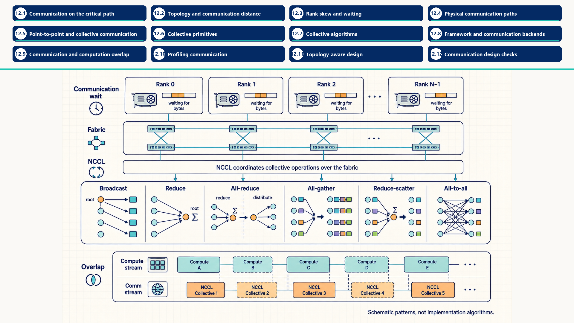
The figure separates the framework process group, NVIDIA Collective Communications Library (NCCL), and physical fabric. Broadcast, reduce, all-reduce, all-gather, reduce-scatter, and all-to-all are drawn as different data relationships rather than as one repeated mesh. The overlap panel shows that communication can share time with independent compute only when dependencies and resources permit it.

The levers this chapter develops, in the vocabulary of Section 1.6.1, are scale out, because dividing dependent work across devices adds communication, and keep the hardware busy, because overlap can hide part of that communication time.

12.1 Communication on the critical path

Single-GPU computation can often be overlapped, fused, compiled, or quantized. Communication is harder because it couples ranks. If one rank reaches a collective late, other ranks may wait. If a tensor-parallel layer needs partial results from peers every token, the interconnect becomes part of the critical path. Communication cost includes bandwidth, latency, topology, synchronization, and software overhead.

• Rank coupling: A distributed operation can force multiple processes to wait at the same logical point. Fast ranks do not finish earlier if they are blocked by slow ranks.
• Critical-path communication: Data movement that must complete before the next useful computation can start. Tensor-parallel collectives in a decode step are often critical-path work.
• Payload size: The number of bytes moved. Large gradients, activation tensors, parameter shards, and expert-routing buffers can dominate bandwidth.
• Startup latency: Fixed cost before useful bytes move. This is important for frequent small messages and per-layer collectives.
• Topology effect: The same collective can be fast or slow depending on whether it stays within NVLink/NVSwitch or crosses node boundaries through NICs and switches.

\[ \text{transfer service time} \approx \text{latency} + \frac{\text{bytes transferred}}{\text{effective bandwidth}} \tag{12.1}\]

Latency is the startup cost for the operation. Bytes transferred is the payload size. This two-term form is often called the latency-bandwidth, or alpha-beta, model: alpha is the startup latency and beta the time per byte. Effective bandwidth is lower than theoretical link bandwidth because algorithms, topology, contention, protocol overhead, and synchronization reduce usable throughput. For example, moving 1 GB over an effective 100 GB/s path with 20 microseconds of startup cost takes roughly 10.02 ms. The approximation omits overlap, algorithmic chunking, rank skew, network contention, and topology-dependent routing.

Message size changes which term dominates. A small collective can be slow because every rank pays startup and synchronization cost. A very large collective can use the fabric efficiently but spend most of its time moving bytes. Middle sizes are often the hardest to reason about because protocol choice, chunking, queueing, and overlap determine whether latency or bandwidth is exposed.

Table 12.1: How message size changes latency and bandwidth cost.

Message-size range	Dominant cost	Typical examples	Useful change
Small and frequent	Startup latency, synchronization, launch overhead, rank skew	Per-layer tensor-parallel collectives, small control tensors, frequent expert routing metadata	Reduce message count, keep traffic in the fast local domain, combine operations when possible
Medium	Transition between latency and bandwidth; protocol and chunking choices matter	FSDP layer all-gathers, moderate gradient buckets, activation transfers	Tune bucket or shard sizes, improve overlap, and inspect backend algorithm choice
Large	Effective bandwidth and topology contention	Large gradient buckets, full-parameter shards, checkpoint or bulk cache movement	Use high-bandwidth paths, hierarchical collectives, compression, or overlap with independent compute

Message size suggests whether startup delay or sustained transfer is the first limit. The route then sets the latency and bandwidth available to that payload, including the device, switch, and node boundaries where links become shared.

12.2 Topology and communication distance

Scalable clusters use switched hierarchy: endpoints connect to local switches, and the fabric routes traffic through switch layers rather than requiring every device pair to have a dedicated cable.

Large clusters often use hierarchical switch designs such as leaf-spine topologies. Leaf switches connect servers in a rack or local group. Spine switches connect leaf groups. The relevant capacity is the bandwidth available when many endpoints communicate across those groups at once.

Bisection bandwidth: The minimum aggregate bandwidth across a division of the network’s endpoints into two equal-sized groups, taking the minimum over all such divisions.¹ The direction convention matters: the example below counts traffic in one direction, without adding the reverse direction’s capacity.

Worked example: Concurrent traffic across a network division

Suppose endpoints A and B are on one side and C and D on the other. A sends to C at 50 GB/s while B sends to D at 50 GB/s. The simultaneous demand across this division is 50 + 50 = 100 GB/s. If the paths share a 60 GB/s upstream limit, their combined rate cannot exceed 60 GB/s, even if each endpoint has a 100 GB/s link. An equal allocation would give each transfer 30 GB/s, although actual sharing depends on routing and scheduling.

Conclusion: One fast endpoint link does not establish sufficient capacity across the division. A leaf-spine design can add parallel paths as the cluster grows, but its achieved capacity depends on uplink provision and concurrent traffic. Section 12.11 connects this constraint to placement and oversubscription (upstream links with less capacity than the endpoints attached below them).

Every extra switch hop adds latency, and shared links can become congested even in a scalable switched design.

Scale-up communication stays inside a tightly coupled accelerator domain with fast GPU-to-GPU paths. That domain is often one server, but rack-scale NVLink systems can join GPUs across more than one compute tray or node. Scale-out communication crosses the cluster network through network interface cards (NICs) and fabrics such as InfiniBand, RDMA over Converged Ethernet (RoCE), or Ethernet. Frequent latency-sensitive traffic such as tensor-parallel collectives should remain inside the fastest available scale-up domain whenever possible.

A direct full mesh is the contrasting limit: every device connects to every other device. Port and cable demand grows rapidly with device count, which is why large systems use switched hierarchy instead.

\[ \text{full-mesh links} = \frac{N(N - 1)}{2} \tag{12.2}\]

A full mesh among N endpoints needs N(N - 1)/2 undirected links, so direct wiring grows quadratically. Leaf-spine and related Clos fabrics replace those dedicated pairwise links with shared switch paths. A host-to-host path can be counted by switches or by physical links. State the convention before describing a path as a particular number of hops.

12.3 Rank skew and waiting

An apparently slow collective can include time spent waiting for another rank before useful transfer finishes. Four quantities help explain the interval: operation startup, the byte rate of the selected path, the topology crossed, and differences in rank readiness. Rank skew: A difference in when participating ranks become ready for the same operation. Section 12.1 estimates startup plus transfer service once the required inputs are ready. Its equation does not estimate the preceding wait for a late rank.

Worked example: Rank waiting and transfer service

Assume two GPU timelines have been aligned to a common time origin. Rank 0 has its input ready and reaches the collective at 2 ms. Rank 1 reaches it at 5 ms. For this illustrative serialized schedule, no useful transfer occurs until 5 ms, and the result becomes available to both ranks at 7 ms. Dependent computation can then start at 7 ms.

Rank 0’s observed entry-to-result interval is 7 - 2 = 5 ms: 3 ms waiting plus 2 ms of collective service. Rank 1 observes 7 - 5 = 2 ms. If startup is 0.02 ms and the modeled per-rank payload is 0.198 GB over an effective 100 GB/s path, the estimate is 0.02 + 1000 x 0.198 / 100 = 2 ms. It models the service interval here, not rank 0’s full 5 ms.

Conclusion: Removing the readiness gap shortens rank 0’s observed collective interval without increasing network bandwidth. These are assumed trace values, not measurements. Real chunked collectives can make partial progress before every rank arrives, so waiting and transfer need not form two separate additive intervals. A local CUDA event pair also does not establish a shared clock across GPUs. Aligned rank traces and dependencies are needed to attribute the delay.

Optimizations target different ingredients. Larger buckets can improve bandwidth efficiency but may reduce overlap. Topology-aware rank placement can keep frequent collectives on fast links. Reducing message count can help latency-bound paths. Removing rank imbalance can shorten apparent collective time without changing the network.

Once the trace separates startup, transfer, and rank waiting, map the slow interval to the actual GPU-to-GPU or GPU-to-NIC path. The fabric and device placement determine which changes can improve it.

12.4 Physical communication paths

Communication fabrics should be described by scope. Some links move bytes inside a server. Some connect servers. Some are general-purpose and some are designed for high-performance GPU communication.

Section 2.6 defines PCIe, NVLink, NVSwitch, InfiniBand, RoCE, and Ethernet. Two of their properties matter once traffic is collective. The pairwise bandwidth of NVLink depends on the GPU model and on whether the selected GPUs are joined directly or through NVSwitch. RoCE performance depends strongly on network configuration, congestion control, and near-lossless behavior, and standard Ethernet paths are often a poor fit for frequent latency-sensitive collectives unless engineered for that workload.

• GPUDirect RDMA: Lets a compatible NIC directly access GPU memory over PCIe instead of staging the payload through host memory, following the NVIDIA GPUDirect RDMA Documentation². The CPU still prepares and submits the communication. Direct access removes a copy path, not all CPU coordination, and it requires compatible GPU, NIC, driver, PCIe topology, and IOMMU settings. An unsupported or poorly connected path can fall back to host staging or perform badly.

Fabric caveat

A fabric name is only the starting point for a performance estimate. Effective bandwidth depends on topology, routing, contention, message size, collective algorithm (the schedule that implements a collective, Section 12.7), and whether the software stack actually uses the intended path.

The critical distinction is local versus remote path. Frequent per-layer traffic is most viable inside a fast GPU fabric. Cross-node traffic additionally traverses a GPU-to-NIC path, a network interface, switches, and the destination path. Product names and peak bandwidth figures are generation-specific, so verify the installed topology and achieved transfer rate rather than copying a nominal number.

12.5 Point-to-point and collective communication

Distributed programs communicate either through explicit pairwise transfers or through group operations. The choice changes both the code structure and the synchronization behavior.

• Point-to-point communication: One rank sends data to another rank. It is common in pipeline stages, custom protocols, explicit activation transfers, and control paths where the communication pattern is irregular.
• Collective communication: A group of ranks participates in one operation with a defined group-level result, such as all-reduce, all-gather, or all-to-all.
• Ordering requirement: Ranks must call compatible collectives in compatible order. Mismatched ordering can hang or corrupt the distributed program.
• Point-to-point versus collective trade-off: Point-to-point communication can be flexible but harder to reason about globally. Collectives are structured and optimized, but they create synchronization points.

The semantics define who participates and which ranks receive results. They do not prescribe a central coordinator or physical traffic path. The next section names the common group transformations before their ring, tree, or hierarchical implementations are considered.

12.6 Collective primitives

A collective operation is a group communication primitive used by strategies such as Distributed Data Parallel (DDP) for gradient synchronization, Fully Sharded Data Parallel (FSDP) for sharded model state, tensor parallelism for layer-internal slices, and expert parallelism for routed token state.

• Broadcast: One source rank sends the same tensor to every other rank. It copies a source value and is commonly used to initialize or synchronize parameters.
• Reduce: Many ranks contribute tensors that are combined on one destination rank. Use Reduce when only one rank needs the combined result. Use all-reduce when every rank needs it.
• All-reduce: All ranks contribute tensors, the tensors are reduced, and every rank receives the reduced result. DDP uses it for gradient synchronization and pays both reduction and redistribution traffic.
• All-gather: Each rank starts with a shard, and all ranks receive the full collection of shards. Materializing sharded parameters or activations creates a full temporary result on every participant.
• Reduce-scatter: Ranks reduce tensors and each rank receives one shard of the reduced result. FSDP and sharded optimizer paths use its combined reduction and partitioning behavior.
• All-to-all: Every rank sends a different slice to every other rank and receives different slices back. Expert-parallel token routing uses this latency-sensitive and topology-sensitive exchange.

The following array trace uses NCCL’s equal-count collective contracts and rank-ordered layouts.³

Worked example: Reduction, collection, and slice exchange

Three ranks use float32 arrays, compatible calls in the same order, and SUM where a reduction is required. Each six-element input has three consecutive two-element chunks, numbered 0, 1, and 2:

Table 12.2: Input held by each rank before the all-reduce.

Rank	Input, shape [6]
0	[1, 2, 3, 4, 5, 6]
1	[10, 20, 30, 40, 50, 60]
2	[100, 200, 300, 400, 500, 600]

Elementwise SUM combines matching positions: the first output is 1 + 10 + 100 = 111, the second is 2 + 20 + 200 = 222, and the complete result is [111, 222, 333, 444, 555, 666]. All-reduce places that shape-[6] result on every rank.

Reduce-scatter starts from the same three shape-[6] inputs. Rank 0 receives [111, 222], rank 1 [333, 444], and rank 2 [555, 666], each with shape [2]. All-gather applied to these shape-[2] shards concatenates them in rank order, giving the shape-[6] result on every rank. It does not add elements again. Each all-gather send count and reduce-scatter receive count is two elements here.

Reduce with root 0 gives only rank 0 the six-element sum. Broadcast with root 0 instead copies rank 0’s original [1, 2, 3, 4, 5, 6] to everyone. For all-to-all on the original inputs, chunk index selects destination: rank 0 receives [1, 2, 10, 20, 100, 200], rank 1 [3, 4, 30, 40, 300, 400], and rank 2 [5, 6, 50, 60, 500, 600]. Each result has shape [6] and source-rank order, with no addition.

Conclusion: Reduction adds matching elements, gathering concatenates rank shards, and all-to-all rearranges destination slices. This example has equal counts and one dtype on all ranks. Uneven routing needs padding or an interface with explicit split sizes rather than assuming this contract covers it.

Expert-parallel all-to-all cost comes from routing token representations, not from the expert MLP arithmetic alone. A rough payload estimate is the number of routed token copies times hidden dimension times bytes per element, split across destination ranks. Top-k routing multiplies token traffic because one token may be sent to more than one expert.

The payload estimate uses these five cost objects:

• Routed tokens: Tokens assigned from each rank to remote expert ranks. Router imbalance creates tail latency when one expert or rank receives too much work.
• Top-k multiplier: The number of experts selected per token, where each expert is one of the feed-forward sub-networks of a mixture-of-experts layer (Section 13.5.1). Top-2 routing can roughly double routed activation traffic before outputs are combined.
• Hidden dimension and dtype: The bytes carried by each token representation. FP16 or BF16 activations move twice the raw bytes of 8-bit activations before metadata or padding.
• Topology distance: Whether routed tokens stay inside a node, rack, or cross-node fabric. All-to-all is sensitive to simultaneous peer paths and aggregate fabric behavior.
• Combine path: The return path that restores original token order after expert execution. Dispatch cost is only half the story when the combine collective is also critical.

\[ \text{ring all-reduce bytes sent per rank} \approx \frac{2(N - 1)}{N} \times \text{tensor}_{\text{bytes}} \tag{12.3}\]

Here N is the number of ranks and tensor_bytes is the size of the tensor being reduced. Under the standard ring model, each rank sends approximately this many payload bytes across reduce-scatter and all-gather and receives the same amount, following the NCCL Tests PERFORMANCE documentation⁴. With 8 ranks and a 1 GiB tensor, the per-rank sent payload is 1.75 GiB. A send-plus-receive accounting convention would report 3.5 GiB. State the convention before converting traffic to bandwidth. The approximation omits latency per chunk, topology, protocol overhead, and overlap with backward computation.

Worked example: Ring chunks and payload traffic

Use the same three arrays and two-element chunks above. The logical ring sends from rank 0 to 1, from 1 to 2, and from 2 to 0. In each round, all ranks send concurrently. This is one valid teaching schedule, not a claim about a particular NCCL run.

1. Reduce-scatter, round 1: Rank 0 sends its chunk 2, [5, 6], to rank 1, which adds [50, 60] to obtain [55, 66]. Rank 1 sends chunk 0, [10, 20], to rank 2, which adds [100, 200] to obtain [110, 220]. Rank 2 sends chunk 1, [300, 400], to rank 0, which adds [3, 4] to obtain [303, 404].
2. Reduce-scatter, round 2: Each rank forwards the partial chunk it just received. Rank 0 sends [303, 404] to rank 1, which adds [30, 40] to obtain its final shard [333, 444]. Rank 1 sends [55, 66] to rank 2, which adds [500, 600] to obtain [555, 666]. Rank 2 sends [110, 220] to rank 0, which adds [1, 2] to obtain [111, 222]. Every final shard now includes all three contributions.
3. All-gather, round 1: Each rank sends its final shard to its successor without further addition. Rank 0 gains chunk 2, rank 1 gains chunk 0, and rank 2 gains chunk 1.
4. All-gather, round 2: Each forwards the newly received shard. Rank 0 gains chunk 1, rank 1 gains chunk 2, and rank 2 gains chunk 0. Placing the chunks in index order gives [111, 222, 333, 444, 555, 666] on every rank.

Each float32 input occupies 6 x 4 = 24 bytes, and each chunk occupies 2 x 4 = 8 bytes. A rank sends two chunks per phase, or 16 bytes for reduce-scatter and 16 bytes for all-gather, totaling 32 bytes. It receives the same amount. For N equal chunks, each phase needs N - 1 rounds carrying tensor_bytes / N per rank per round. Two phases therefore send 2 x (N - 1) / N x tensor_bytes per rank. With N = 8 and a 1 GiB tensor, this is 1.75 GiB sent and 1.75 GiB received.

Conclusion: The two factors of (N - 1) / N come from reducing distributed chunks and then redistributing the completed shards. This is payload accounting, not elapsed time or proof of the selected runtime algorithm. Protocol bytes, latency, topology, rank skew, and overlap still require a trace.

A runtime may select a different ring chunk order, a tree, or a hierarchical algorithm while preserving the same all-reduce result. Its trace establishes the actual schedule.

Collective names specify before-and-after tensor ownership. Their measured cost still depends on the backend’s chosen schedule, chunking, topology, rank readiness, and overlap.

12.7 Collective algorithms

A collective algorithm is the communication schedule used to implement a collective primitive. The same all-reduce request can therefore run as a ring, a tree, or a hierarchy depending on message size, topology, backend heuristics, and runtime settings. The ring versus tree alternative is documented as independent of the requested reduction in the NCCL Tests PERFORMANCE documentation⁵, while hierarchical scheduling means local aggregation inside a fast domain followed by cross-domain exchange and local distribution.

• Ring collective: Streams chunks around ranks and can use bandwidth well for large tensors, especially when each link can stay busy.
• Tree collective: Aggregates through a branching structure and can reduce latency for smaller messages or topologies where a ring would expose too many sequential hops.
• Hierarchical collective: Communicates inside a fast scale-up domain first, then across slower domains, then inside the destination scale-up domain. This matches systems where NVLink/NVSwitch and InfiniBand/RoCE have different costs.
• Topology awareness: Chooses or tunes the schedule using the actual device, switch, and network layout rather than treating every rank pair as equally expensive.

A hierarchical schedule performs local aggregation inside a fast GPU island, exchanges reduced data across the slower inter-node path, and then distributes the result locally. A tree schedule is a different branching reduction and distribution algorithm. A two-node hierarchy should not be labeled as a tree unless the branching parent-child structure is actually shown.

12.8 Framework and communication backends

After the payload, topology, collective semantics, and possible schedules are defined, the software stack can be assigned concrete responsibilities. A distributed strategy decides what must communicate, a framework API expresses the operation for a group of ranks, a backend implements it, and the selected transport carries the bytes over the installed hardware.

• torch.distributed: The PyTorch API for initializing process groups, assigning rank identities, and issuing point-to-point or collective operations.
• Backend: The implementation selected by a process group to execute its communication operations, such as NCCL for many CUDA tensor collectives or Gloo for common CPU/control paths.
• Strategy boundary: DDP, FSDP, tensor parallelism, pipeline parallelism, and expert parallelism decide which objects and operations are required. The API and backend execute those requests.

Backends do not all occupy one interchangeable role. NCCL is commonly selected for CUDA tensor collectives on NVIDIA GPUs, following the NVIDIA Collective Communications Library Documentation⁶ and the torch.distributed documentation⁷. Gloo is commonly used for CPU tensors and control-oriented paths. Message Passing Interface (MPI) implementations provide broader HPC process and communication facilities. Unified Communication X (UCX) exposes transport abstractions used by several distributed-runtime stacks. Compatibility depends on the framework build, tensor location, operation, platform, and deployment configuration.

NCCL (Section 3.1.2) implements the collective operations and chooses algorithms over the available paths, such as PCIe, NVLink, NVSwitch, and network interfaces.

NCCL does not decide the training strategy. It implements communication operations requested by frameworks or distributed libraries. For example, DDP may need all-reduce for gradients, FSDP may need all-gather and reduce-scatter for sharded state, and expert parallelism may need all-to-all routing. NCCL tries to execute those operations efficiently on the hardware topology.

• Process group: A set of ranks that participate in communication. PyTorch creates process groups and calls backend collectives through them.
• Collective algorithm: The pattern NCCL uses to move chunks, such as ring, tree, or hierarchical variants. The selected algorithm depends on message size, rank count, and topology.
• Transport: The path used underneath the collective, such as peer-to-peer GPU links, PCIe, shared memory, sockets, InfiniBand, or RoCE depending on the system.
• NCCL logs: NCCL_DEBUG=INFO and related settings expose backend decisions. Logs are diagnostic evidence, not proof of achieved performance by themselves.

The rank variables used to select local devices and the NCCL settings used to diagnose transports are listed in Section 12.8.1.

A useful debugging question is: did the framework request the intended collective, did NCCL select the intended transport, and did the measured trace show that the collective was on the critical path?

Tracing these responsibilities helps distinguish two diagnostic errors: changing a framework strategy when the wrong network interface was selected, or changing a transport variable when the strategy itself communicates too often for the topology.

12.8.1 Launching ranks and selecting transports

A training job with one process per GPU needs every process to know its identity before any collective can run. The process, rank, and GPU setup in Section 2.5 supplies the mapping used here. Under the one-process-per-GPU assumption, a rank identifies a participating process. RANK is its identity across the whole job, LOCAL_RANK identifies it within its node, and WORLD_SIZE counts participating processes. A collective (Section 12.5) is called by all participating processes in a group.

Worked example: Reading a two-node launch

Assume two nodes, each with two GPUs visible in the same local order to its workers, and one worker process per GPU. On node A, the processes have (RANK, LOCAL_RANK) pairs (0, 0) and (1, 1). On node B they have (2, 0) and (3, 1). Every process has WORLD_SIZE = 4. The program binds each worker to the visible device indexed by its LOCAL_RANK. Rank 2 therefore uses node B’s local device 0, not a device numbered 2 on that node.

The default four-process group can now run a collective: each rank supplies its tensor to the same operation in compatible order. A local rank is reused on different nodes, while a global rank is unique within the job. Comparing these logged pairs with the intended layout checks placement before interpreting communication timing.

torchrun is the usual launch tool for PyTorch distributed jobs. It creates one or more processes and sets rank-related environment variables such as RANK, WORLD_SIZE, and LOCAL_RANK. For diagnosis, NCCL_DEBUG=INFO can expose selected transports and topology decisions, following the torch.distributed documentation⁸. A process group selects the backend implementation, such as NCCL for CUDA tensor collectives or Gloo for CPU paths, while ranks must call compatible collectives in compatible order.

• NCCL_DEBUG=INFO prints NCCL initialization and communication diagnostics.
• NCCL_SOCKET_IFNAME selects the network interface for socket-based NCCL paths.
• NCCL_IB_DISABLE=1 disables NCCL’s InfiniBand/RoCE transport, allowing fallback to another available transport such as IP sockets.⁹
• NCCL_P2P_DISABLE can disable peer-to-peer GPU communication for diagnosis.

For reproducible comparisons, set diagnostic environment variables before launching workers and use a fresh run for each configuration. Do not rely on changing an environment variable to reconfigure an existing communicator. These settings can test routing hypotheses, but they do not choose the model’s sharding strategy or prove that the enabled path reaches peak throughput.¹⁰

12.9 Communication and computation overlap

Communication/computation overlap means scheduling data movement so it occurs while independent useful computation is still running. It can reduce step time by shortening the communication interval that remains exposed, even when a tail still lies on the critical path. Resource contention can offset that gain, so the end-to-end time must be measured.

• DDP overlap: Buckets gradients and launches all-reduce during backward propagation when a bucket is ready and earlier buckets in the required reduction order have been launched.
• FSDP overlap: Can prefetch or all-gather parameters near the layer that needs them.
• Pipeline overlap: Runs micro-batches across stages so some stages compute while others transfer activations or gradients.
• Tensor-parallel limits: Layer-internal collectives often have little independent work after them, so they are harder to hide than DDP gradient buckets.
• Serving limits: Decode has a short per-token critical path, so communication in tensor-parallel serving can be visible even when training overlap looks good.

Overlap works only when there is independent computation available while communication runs. If the next layer or token needs the communicated result immediately, the communication remains exposed.

Adjacent compute and collective blocks do not prove overlap. When compute and communication lanes are aligned, they expose the end-to-end critical path. If shortening the collective would shorten the step, its remaining tail is exposed. Otherwise, independent computation has hidden it.

12.10 Profiling communication

Communication profiling asks where time is lost when ranks exchange tensors. The evidence can come from several layers: the framework call such as dist.all_reduce, the NCCL backend that chooses a collective algorithm and transport, the GPU timeline that shows copy or collective kernels, the network fabric that carries bytes between nodes, and the rank synchronization behavior that makes fast ranks wait for slow ranks.

When communication is suspected, a dedicated distributed harness separates the collective from model computation. The template below warms the operation, measures repeated all-reduces on every rank, reports the slowest rank’s mean time, and converts the ring traffic estimate into an effective per-rank payload rate.

Worked example: NCCL collective timing probe

This distributed probe shows the objects involved in a simple all-reduce: process group, rank-assigned GPU, tensor payload, synchronization, and elapsed time. It requires a CUDA/NCCL-enabled PyTorch installation and at least two available GPUs, and is launched with torchrun across the intended number of GPUs. Its tensor payload is 512 MiB per rank before communication and checking buffers. Each warmup and timed all-reduce starts from a known payload value. The final result of each loop is checked for finite values and the expected world-size sum outside the recorded timing intervals.

Code example: NCCL collective timing probe

import os
import torch
import torch.distributed as dist

dist.init_process_group("nccl")
try:
    local_rank = int(os.environ["LOCAL_RANK"])
    torch.cuda.set_device(local_rank)
    device = torch.device("cuda", local_rank)
    payload = torch.zeros(256 * 1024 * 1024, device=device, dtype=torch.float16)
    world = dist.get_world_size()

    for _ in range(5):
        payload.fill_(1.0)
        dist.all_reduce(payload, op=dist.ReduceOp.SUM)
    torch.cuda.synchronize()
    assert torch.isfinite(payload).all(), "Non-finite result in warmup"
    assert (payload == world).all(), "Incorrect all_reduce result"
    dist.barrier()

    samples_ms = []
    for _ in range(20):
        payload.fill_(1.0)
        start = torch.cuda.Event(enable_timing=True)
        stop = torch.cuda.Event(enable_timing=True)
        start.record()
        dist.all_reduce(payload, op=dist.ReduceOp.SUM)
        stop.record()
        stop.synchronize()
        samples_ms.append(start.elapsed_time(stop))
    assert torch.isfinite(payload).all(), "Non-finite result in measured loop"
    assert (payload == world).all(), "Incorrect all_reduce result"

    mean_ms = torch.tensor(sum(samples_ms) / len(samples_ms), device=device)
    dist.all_reduce(mean_ms, op=dist.ReduceOp.MAX)
    ring_bytes = 2 * (world - 1) / world * payload.numel() * payload.element_size()
    effective_gb_s = ring_bytes / (mean_ms.item() / 1000) / 1e9

    if dist.get_rank() == 0:
        print(f"slowest_rank_mean_ms={mean_ms.item():.3f}")
        print(f"estimated_ring_payload_GBps={effective_gb_s:.1f}")
finally:
    dist.destroy_process_group()

The probe isolates one payload and one collective, so it can compare rank placement or transport configurations without model noise. NCCL_DEBUG=INFO can reveal selected interfaces and topology decisions, but only the timed samples and system trace show achieved behavior. Compare the result with a topology-aware theoretical estimate and an Nsight Systems trace before assigning the gap to the fabric.

PyTorch Profiler can show collective operators in the framework trace. Nsight Systems shows whether collectives overlap kernels or sit on the critical path. NCCL logs help diagnose backend selection, network interface choice, peer-to-peer paths, and failures.

12.11 Topology-aware design

Topology-aware distributed design means choosing a parallelism and serving architecture that matches how often tensors must move. A topology defines which transfers are cheap enough to place on the critical path.

The central rule is communication frequency versus distance. The more often a tensor must move, the closer the communicating devices should be. Per-token and per-layer communication should stay inside the fastest scale-up domain whenever possible. Per-step communication can sometimes cross nodes when overlap and bandwidth are good. Background movement can use slower tiers if it does not block the hot path.

• Scale-up domain: A tightly connected GPU group such as one server, pod, or NVLink/NVSwitch island. It is the preferred place for frequent tensor-parallel or decode-critical communication.
• Scale-out domain: Multiple nodes connected through NICs and switches. It provides capacity and aggregate throughput, but it usually adds latency, routing, and contention.
• GPU/NIC affinity: The locality relationship between a GPU and the network card used for cross-node traffic. Poor affinity can add PCIe hops, CPU-socket crossings, or host staging.
• Bisection bandwidth: The capacity across the equal-sized endpoint groups defined in Section 12.2. Concurrent transfers share this capacity, so a fast single link does not establish the aggregate rate.
• Oversubscription: A topology condition where the upstream fabric has less bandwidth than the sum of attached endpoints. It is common in cost-controlled networks and can hurt concurrent collectives.
• Placement policy: The scheduler or launch decision that maps ranks, serving groups, workers, or replicas onto physical GPUs and nodes.

After those topology objects are named, communication frequency can be matched to distance:

• Per-token communication: Decode-time tensor parallelism, expert routing, logits exchange, or KV movement. It is the most latency-sensitive traffic and should usually stay inside a fast scale-up domain.
• Per-layer communication: Tensor-parallel all-reduce, all-gather, or reduce-scatter inside transformer layers benefits from NVLink, NVSwitch, or an equivalent low-latency scale-up fabric. FSDP and fully sharded Zero Redundancy Optimizer (ZeRO) can also gather parameters around each wrapped unit’s use, rather than communicating only at the optimizer step. The gather frequency depends on how long the policy retains full parameters, as explained in Section 13.4.
• Per-step communication: DDP synchronizes gradient buckets for an update, and ZeRO synchronizes the state required by its sharding stage. Backward computation can overlap some of this traffic. Gradient accumulation changes which micro-batches synchronize. Pipeline stages exchange activations, and backward activation gradients during training, for each micro-batch. Decode pipelines exchange activations on each token step.
• Per-request communication: Request routing and prefill/decode handoff. The acceptable distance depends on time to first token (TTFT), time per output token (TPOT), and tail-latency targets.
• Background communication: Checkpointing, model loading, cache spill/fill, and slow-tier movement. It can use slower paths when the work is amortized and kept off the hot path.

Table 12.3 applies those communication frequencies to complete placement and scheduling patterns. Each row states the intended topology fit and the failure that appears when the mapping is wrong.

Table 12.3: Distributed system design patterns for communication-heavy workloads.

Design pattern	Communication pattern	Topology fit	Failure mode
Topology-aware placement	Ranks with frequent exchange are placed near each other	Prefer NVLink/NVSwitch for frequent collectives; same-rack placement only helps when the measured network path meets the workload’s latency target	Scheduler spreads hot ranks across slow paths
Hierarchical collective	Communicate inside one scale-up domain, then across slower domains, then inside the destination scale-up domain	Matches intra-node GPU fabric plus cross-node network	Treats all rank pairs as equally cheap
Bucket and overlap	Group tensors and launch communication while compute continues	Works when independent compute remains	Small buckets add overhead; large buckets expose a tail
Shard-and-gather	Store state sharded; materialize only near layer use	Works when gather/reduce paths are fast enough	Memory saved locally becomes network-bound
Scale-up first, scale-out second	Keep per-token or per-layer traffic inside one node/group	Serving replicas or groups scale across nodes	Cross-node tensor parallelism hurts TPOT
Sticky KV-cache placement	Route active requests near the GPUs holding their KV cache	Serving groups with stable cache locality	Load balancing moves cache-heavy requests too freely
Rail or NIC-aware grouping	Ranks that leave a node use the intended NIC path	Systems with multiple NICs or network rails	Traffic concentrates on one weak interface
Topology-aware replica placement	Replicas are spread to avoid shared-fabric hot spots	Serving fleets and multi-tenant clusters	All replicas contend on the same leaf or spine

Design checklist

Object: Is the moving object a gradient, parameter shard, activation, KV block, expert token, logits vector, request, or checkpoint chunk?

Frequency: Does it move per token, per layer, per step, per request, or in the background?

Critical path: Would shortening this transfer reduce TTFT, TPOT, step time, or tail latency?

Overlap: Is there independent compute available while the transfer runs?

Locality: Does the traffic stay inside the intended scale-up domain, or does it cross NICs and switches?

Contention: What happens when multiple jobs, collectives, or serving replicas share the same fabric?

Metric: Is success judged by throughput, TTFT, TPOT, tail latency, utilization, memory capacity, or cost?

Comparing these patterns helps expose a common distributed-system error: choosing a parallelism strategy because it fits memory, then discovering that its communication frequency does not fit the topology. Memory capacity and communication distance have to be designed together.

12.12 Communication design checks

Reliable distributed diagnosis names the framework call, backend library, physical path, and critical-path wait. The following checklist establishes the evidence before a communication strategy changes.

Checklist: Communication design

• NVLink, a physical GPU interconnect, is distinguished from NCCL, a collective communication library.
• torch.distributed is identified as the framework API that calls a backend. The backend and selected transport remain separate evidence items.
• Tensor-parallel groups remain on the fastest available links when each layer requires frequent communication.
• Rank placement reflects topology so a local collective does not cross an unnecessary slow path.
• Collective timing is synchronized and warmup remains separate from steady-state measurement.

With the communication primitives and physical paths defined, Chapter 13 can compare distributed training and inference strategies by the tensors they exchange, the frequency of those exchanges, and the topology that carries them.

---

1. Bindel, D. (2015, October 6). Distributed memory: Networks and models. Cornell University, CS 5220 course notes, Network properties. https://www.cs.cornell.edu/~bindel/class/cs5220-f15/slides/2015-10-06-network.html. Supports the minimum-capacity equal-division definition. The four-endpoint rates in this chapter are assumed teaching inputs, not benchmark results.

2. NVIDIA. (2026). GPUDirect RDMA Documentation (v13.4). https://docs.nvidia.com/cuda/gpudirect-rdma/. Supports direct data exchange between GPU and third-party PCIe peer such as a NIC, with address translation through the NVIDIA kernel driver, while CPU libraries prepare and submit transfers. Limit: peers must share a compatible PCIe root complex path, IOMMU must allow the mapping, and topology, BAR size, and platform support determine whether the direct path is available or falls back.

3. NVIDIA. (2026). NVIDIA Collective Communications Library Documentation (NCCL 2.32.3). https://docs.nvidia.com/deeplearning/nccl/user-guide/docs/index.html. This current-documentation URL can change versions. Supports NCCL as the common GPU collective library implementing AllReduce, Broadcast, Reduce, AllGather, ReduceScatter, AlltoAll, Gather, Scatter, and point-to-point operations over paths including PCIe, NVLink, NVSwitch, and network interfaces. Limit: documents library behavior and configuration, not achieved bandwidth; algorithm choice depends on message size, rank count, topology, and settings such as NCCL_ALGO.

4. NVIDIA. (2024). NCCL Tests PERFORMANCE Documentation. Pinned commit c6eb15875f508076f3f26de4f7da3899701bc4db dated 2024-07-25 at https://raw.githubusercontent.com/NVIDIA/nccl-tests/c6eb15875f508076f3f26de4f7da3899701bc4db/doc/PERFORMANCE.md, commit page at https://github.com/NVIDIA/nccl-tests/commit/c6eb15875f508076f3f26de4f7da3899701bc4db. Supports AllReduce bus-bandwidth correction factor 2 times (n minus 1) divided by n, and (n minus 1) divided by n for ReduceScatter and AllGather, with the AllReduce reduction described as independent of ring, tree, or other point-to-point algorithm. Limit: factor converts algorithm bandwidth to bus bandwidth and does not prove which schedule a runtime selects or what elapsed time a topology achieves.

5. NVIDIA. (2024). NCCL Tests PERFORMANCE Documentation. Pinned commit c6eb15875f508076f3f26de4f7da3899701bc4db dated 2024-07-25 at https://raw.githubusercontent.com/NVIDIA/nccl-tests/c6eb15875f508076f3f26de4f7da3899701bc4db/doc/PERFORMANCE.md, commit page at https://github.com/NVIDIA/nccl-tests/commit/c6eb15875f508076f3f26de4f7da3899701bc4db. Supports AllReduce bus-bandwidth correction factor 2 times (n minus 1) divided by n, and (n minus 1) divided by n for ReduceScatter and AllGather, with the AllReduce reduction described as independent of ring, tree, or other point-to-point algorithm. Limit: factor converts algorithm bandwidth to bus bandwidth and does not prove which schedule a runtime selects or what elapsed time a topology achieves.

6. NVIDIA. (2026). NVIDIA Collective Communications Library Documentation (NCCL 2.32.3). https://docs.nvidia.com/deeplearning/nccl/user-guide/docs/index.html. This current-documentation URL can change versions. Supports NCCL as the common GPU collective library implementing AllReduce, Broadcast, Reduce, AllGather, ReduceScatter, AlltoAll, Gather, Scatter, and point-to-point operations over paths including PCIe, NVLink, NVSwitch, and network interfaces. Limit: documents library behavior and configuration, not achieved bandwidth; algorithm choice depends on message size, rank count, topology, and settings such as NCCL_ALGO.

7. PyTorch. (2026). Distributed Communication Package: torch.distributed. Versioned v2.14 documentation at https://docs.pytorch.org/docs/2.14/distributed.html, created 2017-07-12 and updated 2026-08-07. Supports process groups with rank identity, backend selection with NCCL for CUDA collectives and Gloo for CPU paths, and NCCL debugging with NCCL_DEBUG equals INFO. Limit: backend availability depends on build and platform; the page documents API behavior, not achieved performance.

8. PyTorch. (2026). Distributed Communication Package: torch.distributed. Versioned v2.14 documentation at https://docs.pytorch.org/docs/2.14/distributed.html, created 2017-07-12 and updated 2026-08-07. Supports process groups with rank identity, backend selection with NCCL for CUDA collectives and Gloo for CPU paths, and NCCL debugging with NCCL_DEBUG equals INFO. Limit: backend availability depends on build and platform; the page documents API behavior, not achieved performance.

9. NVIDIA. (NCCL 2.32.3 documentation). Environment Variables. Retrieved September 28, 2026, from https://docs.nvidia.com/deeplearning/nccl/user-guide/docs/env.html. Describes diagnostic settings and InfiniBand/RoCE transport disabling. The current-documentation URL can change versions. Starting a fresh run for each configuration is a conservative test procedure used here, not a documented guarantee about when every setting is read or whether an existing communicator is reconfigured.

10. NVIDIA. (NCCL 2.32.3 documentation). Environment Variables. Retrieved September 28, 2026, from https://docs.nvidia.com/deeplearning/nccl/user-guide/docs/env.html. Describes diagnostic settings and InfiniBand/RoCE transport disabling. The current-documentation URL can change versions. Starting a fresh run for each configuration is a conservative test procedure used here, not a documented guarantee about when every setting is read or whether an existing communicator is reconfigured.