9  Decode and KV Cache

Explain why decode performance depends on cache growth, memory layout, batching, and kernel shape, then connect those mechanisms to measured throughput and latency.

Decode optimization focuses on the repeated one-token step. A small inefficiency in one step becomes large when repeated for thousands of generated tokens across many active requests. Decode is therefore a scheduling, memory-layout, and cache-management problem as much as a model-forward problem.

The key-value cache avoids recomputing the full prefix, but it also becomes the largest dynamic memory object in long-context serving. Cache layout determines whether decode kernels read memory efficiently. Allocation policy determines how many requests can be admitted without waste.

A useful diagnostic path compares naive recomputation with cached decode, inspects weight and KV traffic, and then tests launch, layout, paging, or batching changes against the measured limit. A more elaborate path is not automatically faster: metadata, indirection, compilation, and scheduling overhead can outweigh its benefit for small workloads.

The figure below compares how a cache can be allocated as requests grow.

Figure 9.1: Decode reuses projected key and value state but still reads a growing attention history.

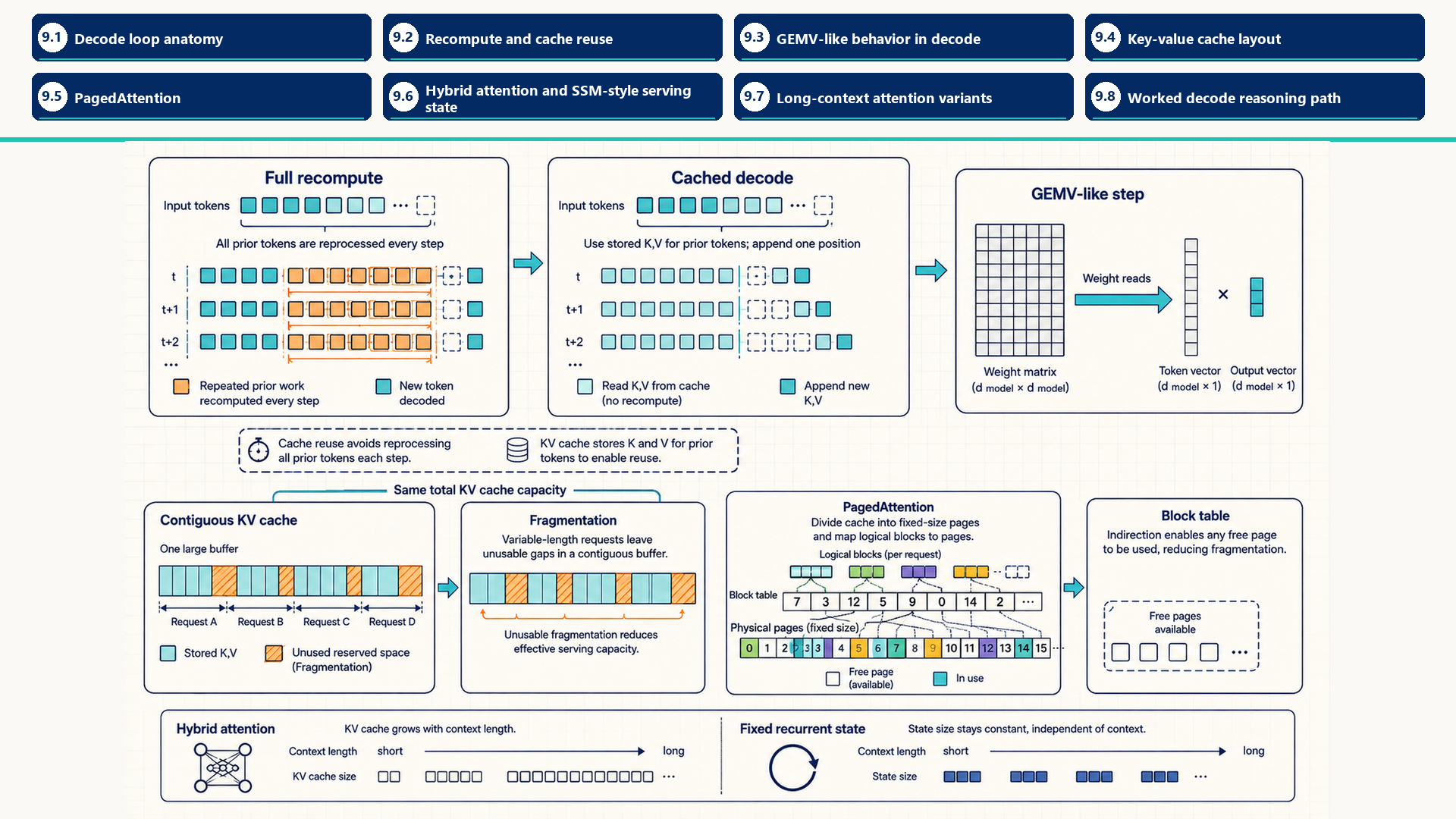
The allocation panels separate logical token order from physical placement. Contiguous reservation can waste free space between requests. A block table can map logical blocks to non-contiguous physical blocks, trading less over-reservation for metadata, indirection, and final-block waste. Fixed recurrent state is a different model design, not another KV layout.

The levers this chapter develops, in the vocabulary of Section 1.6.1, are do less work, because the KV cache removes the recomputation of earlier tokens, move fewer bytes, because layout decides what each decode step reads, and fit in memory, because paging decides how many requests stay resident.

9.1 Decode loop anatomy

Autoregressive generation uses prefill to predict the first output token, then decode steps to predict later tokens. A naive loop may rerun the model over the growing prefix. Let the prompt contain \(P\) tokens and let the model generate \(G\) new tokens without a cache. The first generation pass processes \(P\) tokens. Later passes process every prefix length from \(P+1\) through \(P+G-1\). Across all \(G\) outputs, projection and other per-token layer work therefore processes

\[ \sum_{j=0}^{G-1}(P+j)=GP+\frac{G(G-1)}{2} \]

token positions. Dense full-prefix attention accumulates work proportional to

\[ \sum_{j=0}^{G-1}(P+j)^2=GP^2+PG(G-1)+\frac{G(G-1)(2G-1)}{6}. \]

This becomes cubic in \(G\) only when generated length grows large relative to the fixed prompt. Caching avoids repeating the old key and value projections, but each new query still attends to a growing history. After prefill, the \(j\)th single-token decode call attends to \(P+j\) positions, including its current input token.

Worked example: Cached decode loop

This runnable example takes a loaded model, input token IDs, and a requested new-token count as input. It returns concatenated generated token IDs for a fixed-length greedy decode decision. It assumes unpadded, equal-length prompts and a compatible Hugging Face Transformers model in evaluation mode (model.eval()) whose forward method accepts past_key_values and infers positions from the growing cache. Padded batches and models with explicit cache-position APIs need additional masks and position arguments. This is not a universal generation wrapper. A zero-token request returns an empty output without running the model. Otherwise, prefill predicts the first output token and creates the cache. Each later call consumes the previous token, reads the cache, and predicts the next token. The loop generates a fixed number of tokens without early stopping at an end-of-sequence token.

Code example: Cached decode loop

import torch

@torch.inference_mode()
def cached_decode(model, input_ids, max_new_tokens):
    if max_new_tokens <= 0:
        return torch.empty((input_ids.size(0), 0), dtype=input_ids.dtype, device=input_ids.device)
    
    out = model(input_ids, use_cache=True)
    past = out.past_key_values
    token = out.logits[:, -1].argmax(dim=-1, keepdim=True)
    generated = [token]

    for _ in range(max_new_tokens - 1):
        out = model(token, past_key_values=past, use_cache=True)
        past = out.past_key_values
        token = out.logits[:, -1].argmax(dim=-1, keepdim=True)
        generated.append(token)

    return torch.cat(generated, dim=1)

The return value contains only generated token IDs, not the original prompt. Attention still reads a cache that grows with context length, so removing prefix recomputation does not make each step constant-cost. The remaining work is often sensitive to memory bandwidth and per-step launch overhead.

9.2 Recompute and cache reuse

Decode implementations trade one cost for another. The three variants below move from recomputation to persistent state and then to runtime-managed execution, but their ranking depends on request size, batch, cache pressure, and implementation overhead.

• Naive decode: Every new token recomputes attention over the whole prefix from scratch. It is simple but quickly becomes wasteful because history is processed repeatedly.
• Cached decode: The model stores key and value tensors from previous tokens. Each new step processes only the newest token and attends to cached history, trading recomputation for persistent memory reads.
• Optimized decode: The serving stack reduces launch overhead, improves batching, lays out cache reads efficiently, pages KV memory, and avoids allocator churn.
• Main trade-off: Caching reduces compute but creates a large dynamic memory object. Optimizing decode is therefore both a kernel problem and a memory-management problem.

This progression explains why a cached loop can be much faster than naive recomputation while still performing poorly in production. Once recomputation is gone, decode is often limited by reading weights and KV cache, maintaining enough active sequences, and launching repeated small steps without CPU gaps.

9.3 GEMV-like behavior in decode

A model can have high theoretical FLOP/s during prefill and still produce slow tokens during decode because workload shape and model size determine whether decode maps to a compute-rich matrix-matrix multiply (GEMM) or to a bandwidth-sensitive path that behaves like a matrix-vector multiply (GEMV).

Section 3.7 defined GEMM and GEMV, and Section 2.8 showed why their arithmetic intensity differs. The distinction matters because matrix-matrix work reuses loaded weights across many output columns, while matrix-vector work often reads many weights for only one or a few token vectors.

• GEMV-like decode: A small-batch decode step multiplies large projection matrices by one or a few token vectors. Weight reuse is low, so arithmetic intensity is low.
• GEMM-like prefill: Prompt processing uses many token positions at once, so the same weights can be reused across a larger matrix of activations. This is usually better for tensor-core utilization.
• Bandwidth implication: Small-batch decode may be dominated by reading model weights and KV cache rather than by raw arithmetic throughput.
• Batching implication: Continuous batching and grouped requests can make the decode step less vector-like by increasing useful work per launch, but they are constrained by latency and KV-cache capacity.

The whole decode step follows the reasoning of Section 2.8. For a dense model whose weights must be fetched from HBM each step, an ideal batch-size-one pass reads each required weight once to produce one token, so the time per token cannot be shorter than the weight bytes divided by the HBM bandwidth. The KV cache adds its own bytes, and those bytes are normally separate for each sequence unless the engine reuses shared-prefix blocks.

Worked example: The decode-step floor for an 8B model

Inputs: A Llama 3 8B-class model (Section 1.1) holds \(8\times10^9\) BF16 parameters, or 16 GB, and its KV cache takes 131,072 bytes per retained token (Section 1.3). An H100 SXM reads HBM at 3.35 TB/s. The estimate ignores activations and assumes that every byte is read once at full bandwidth, so real steps are slower.

Table 9.1: Decode step-time floor for different numbers of sequences and tokens each.

Sequences \(B\)	Tokens each \(T\)	Weight bytes	KV bytes	Step-time floor	Ideal tokens/s ceiling, all sequences
1	8,192	16.0 GB	1.07 GB	5.1 ms	196
32	2,048	16.0 GB	8.6 GB	7.3 ms	4,360
32	8,192	16.0 GB	34.4 GB	15.0 ms	2,129
345	2,048	16.0 GB	92.6 GB	Not admitted on 80 GB	Not admitted on 80 GB

Arithmetic check: At \(B=32\) the weight multiplications need \(2\times8\times10^9\times32\approx5.1\times10^{11}\) FLOPs, about 0.52 ms at the 989 TFLOP/s peak. The step floor is 7.3 to 15.0 ms, so memory traffic sets the larger ideal floor in this model. A measured run can still be limited by launch overhead, inefficient kernels, or scheduling.

Conclusion: In this ideal model, batching shares one read of the weights among all sequences. The tabulated time floors give throughput ceilings: their ratios are about 11 to 22, while each request’s modeled token interval rises from 5.1 ms to 7.3 or 15.0 ms. Actual batching gains require measurements. The weight multiplications would reach the ridge point only near 345 sequences (Section 2.8), but 345 sequences of 2,048 tokens need 92.6 GB of cache, more than one 80 GB GPU holds. For these model shapes and retained lengths, KV-cache capacity can limit the decode batch before the arithmetic units become the limit.

Attention does not improve with batching the way the weight multiplications do. For each cached token, the 32 query heads of a Llama 3 8B layer perform \(4\times32\times128\) FLOPs (a score and a weighted sum per query head) on \(2\times8\times128\times2\) bytes of keys and values. That is 4 FLOP per byte whatever the batch size, far below the ridge point. Long-context decode therefore stays memory-bound in attention. The levers are fewer or smaller cache entries: grouped-query attention (Section 8.6), KV-cache quantization (Section 8.7.1), and the long-context variants of Section 9.7.

9.4 Key-value cache layout

Long-context decode streams a growing key-value cache, so layout decides both whether attention kernels read efficiently and how many requests fit in memory.

Key-value cache layout is the physical organization of cached key and value tensors in GPU High Bandwidth Memory (HBM). It specifies how layers, sequences, token positions, heads, and head dimensions are ordered, and how the serving engine finds the cache blocks for each active request during attention.

• Layer dimension: Each transformer layer stores its own key and value tensors because attention state is layer-specific.
• Sequence and token dimensions: The cache must preserve token order for each request, even when physical blocks are not contiguous.
• Head and head-dimension layout: The arrangement of KV heads and per-head vector elements affects whether attention kernels can read contiguous addresses.
• Append path: Each token processed by a cached model call adds new keys and values. Selecting the next token alone does not append it. The layout must make this write path cheap enough for repeated decode steps.
• Read path: Every decode step rereads prior keys and values for attention. This read path is often more important than append cost for long contexts.
• Block table: Paged layouts add metadata mapping logical token blocks to physical cache blocks, trading lookup indirection for lower memory waste.

A cache layout should support coalesced reads by attention kernels, efficient append of new keys and values, and fast lookup for each active sequence. Grouped-query attention reduces the number of key-value heads and therefore cache size. Quantizing the cache can reduce bandwidth, but only if the attention path supports the format efficiently.

One word, four meanings: cache

Hardware cache: the L1 and L2 storage between the SMs and HBM (Section 2.3). Software influences it through access patterns and supported cache hints or persistence controls, while hardware still manages cache-line placement and eviction¹.

KV cache: the keys and values kept in HBM so that a decode step does not recompute the whole prefix (Section 9.1). The serving engine decides what stays there, which is why layout, block size, and paging policy are optimization objects at all.

Prefix cache: KV blocks kept after a request finishes so that a later request with the same opening tokens can reuse them (Section 10.5).

External KV cache layer: KV blocks moved out of GPU memory into host memory or storage, to be fetched back when needed (Section 10.5.3).

Only the first is hardware-managed. The other three are engine policy, and they are where the decisions in this chapter and the next are made.

KV blocks usually live in HBM and are reread by attention kernels at every decode step. The L2 cache may help when accesses are nearby or repeated, but long-context decode can stream through more KV data than the hardware cache holds, so the reliable objects to change are KV layout, block size, paging policy, attention-kernel tiling, and request locality.

9.5 PagedAttention

PagedAttention is a KV-cache management technique that maps logical token blocks in a sequence to reusable physical KV-cache blocks in GPU memory². The idea is similar to virtual memory: a request has an ordered logical sequence, while the engine is free to place the underlying physical blocks wherever capacity is available.

The problem is variable sequence length. If an engine reserves one large contiguous KV region for the maximum possible output length of every request, short completions leave unused space and long-running service can fragment memory. Paging reduces this waste by allocating fixed-size blocks on demand.

Figure 9.2: Contiguous key-value allocation can waste memory

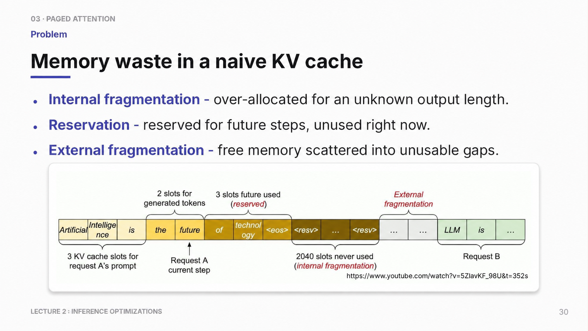
In Figure 9.2, the empty regions represent capacity wasted by a naive policy that reserves a maximum-length contiguous KV region for each request. Other contiguous allocators may reserve less and have different waste patterns.

Paging allocates reusable physical blocks on demand and reduces fragmentation and tail waste³. It does not remove all waste: partially filled final blocks, block tables, metadata work, and indirect kernel addressing remain.

The block table is the central mechanism. Each request has a logical sequence of KV blocks: block 0, block 1, block 2, and so on. The engine maps those logical blocks to physical blocks in GPU memory. For example, request A may map logical blocks [0, 1, 2] to physical blocks [7, 2, 15]. Attention kernels use this mapping to gather the right keys and values even though the physical allocation is non-contiguous.

Blocks are allocated on demand as tokens are generated. This reduces waste because the engine does not need to reserve the maximum possible output length for every request at admission time. In the ideal case, all full blocks are packed and only the final block of an active sequence is partially empty. The trade-off is indirection: every request needs block-table metadata, and kernels or scheduler code must resolve logical positions to physical blocks.

Table 9.2: Contiguous key-value allocation versus paged allocation.

Dimension	Contiguous allocation	PagedAttention-style allocation
Memory reservation	Often reserves for maximum or estimated length	Allocates fixed-size blocks as needed
Fragmentation	Can waste space for short outputs	Reduces waste through block reuse
Lookup	Simple pointer arithmetic	Block-table indirection
Scheduler complexity	Lower	Higher, because block assignment must be tracked

Paged allocation is most useful when variable request lengths make contiguous reservation waste enough HBM to limit admission. It changes cache allocation and lookup, not the attention formula, so kernel efficiency, scheduler fairness, and prefix-cache correctness remain separate measurements.

Paging also allows the engine to run out of free blocks while requests are still generating, because each running request keeps requesting new blocks. The engine must then stop some running requests and release their blocks, a step called preemption. vLLM 0.6.4 (an open-source serving engine, Section 10.1) recomputes a preempted request’s KV cache once space becomes available again and warns that preemption can affect latency. Its documentation suggests more cache memory (gpu_memory_utilization), fewer concurrent sequences or batched tokens (max_num_seqs, max_num_batched_tokens), or more tensor parallelism.⁴ The PagedAttention design also describes swapping, which copies the evicted blocks to CPU memory and back, trading PCIe traffic for recomputation. Recomputation can take less time than the original generation, because the prompt and the tokens generated so far are processed together as one prefill.⁵ Either way, preemption appears as latency spikes for the affected requests, so its rate belongs on the serving dashboard (Section 10.8).

Worked example: PagedAttention block lookup

This pseudocode shows the mapping idea without tying it to a particular engine implementation. The request grows in logical token order, but physical KV blocks do not need to be contiguous. The attention path pays an indirection cost to reduce allocation waste. Paging improves memory management, not the arithmetic complexity of attention. The key point is that logical sequence positions are resolved through a block table before the attention kernel reads KV memory.

Code example: PagedAttention block lookup

block_size = 16
# request A: logical block -> physical KV block
block_table = {0: 7, 1: 2, 2: 15}

def physical_location(token_index):
    logical_block = token_index // block_size
    offset = token_index % block_size
    physical_block = block_table[logical_block]
    return physical_block, offset

The pseudocode implements only metadata translation from a logical token position to a physical block and offset. A complete implementation also accounts for layer, KV head, vector dimension, append writes, vectorized reads, and the attention kernel that consumes the resolved addresses. Conclusion: Block lookup trades indirection for less reserved capacity. Admission and latency measurements show whether that trade-off helps the workload.

9.6 Hybrid attention and SSM-style serving state

In a hybrid model that mixes attention layers with state-space or recurrent layers, attention layers still store one key and value record per retained token, so their state and read traffic grow with context length. The state-space or recurrent layers instead update a fixed-size hidden state for each sequence. In this architecture family, replacing some attention layers with recurrent layers can therefore reduce long-context KV capacity and bandwidth, but it changes the work rather than removing it. These objects are architecture-specific: the model and runtime documentation defines their scan or recurrent-update kernels, state layout, chunking, invalidation, and prefix rules. The recurrent state is a compressed summary, not an addressable record of every past token.

For a recurrent layer, the current token’s input features and the previous hidden state determine a new state and an output for the next layer. The worker reads the old state, computes the update, and retains the new state in its place. A state-space model (SSM) uses a structured state update and an output mapping. Selective SSMs such as Mamba allow parts of those mappings to depend on the current input⁶. The following fixed-coefficient recurrence isolates the storage behavior. It is not a complete Mamba block, a token predictor, or a model-quality comparison.

Worked example: Two tokens and a fixed state

Inputs and task: In inference mode, let \(x_t\) be one scalar feature of token \(t\), rather than its vocabulary ID. The old state is a two-element vector \(h_{t-1}\), initially \(h_0=(0,0)\). Use fixed update rules \(h_{t,1}=0.5h_{t-1,1}+x_t\) and \(h_{t,2}=0.25h_{t-1,2}+2x_t\). The layer output is the scalar \(y_t=h_{t,1}+h_{t,2}\). The question is what must remain stored after processing features \(x_1=2\) and \(x_2=1\).

1. At token 1, the retained contribution from \(h_0\) is \((0,0)\) and the input contributes \((2,4)\). The new state is \(h_1=(2,4)\) and the output is \(y_1=6\).
2. At token 2, the old state contributes \((0.5(2),0.25(4))=(1,1)\) and the new input contributes \((1,2)\). The new state is \(h_2=(2,3)\) and the output is \(y_2=5\). It replaces \(h_1\) for subsequent recurrent execution.

Conclusion: The state still has two elements, but both contain contributions from earlier input. The worker retains \(h_2\), not a list of \(h_0,h_1,h_2\). An attention layer retaining these two token positions instead adds two KV records, \((k_1,v_1)\) and \((k_2,v_2)\), to its history. Fixed state shape limits recurrent storage growth but does not preserve separately addressable token records or establish equivalent model quality.

Prompt processing has all prompt inputs available. A scan computes the sequence of states obtained by applying the update through each input prefix. Suitable affine updates can be composed and evaluated with a parallel scan while preserving those dependencies. Single-token decode has only the newest input and carried state, so it performs one recurrent update. Chunked prompt execution passes the final state of one chunk into the next⁷.

Mamba-style serving therefore shifts attention toward scan kernels, recurrent updates, chunking, and state layout. Fixed recurrent state describes retained inference state per sequence and layer. It does not mean prompt outputs, temporary workspaces, or training activations take constant total memory. Hybrid models still retain growing KV history in their attention layers, and actual runtimes may also keep other architecture-specific state.

9.7 Long-context attention variants

The worked example in Section 9.3 showed that, at long contexts, the KV cache can outweigh the weights in both capacity and bytes read per step. Standard attention stores and rereads a key and a value for every retained token in every layer. Several design families reduce that state. They differ in whether they change the model, which must then be trained or adapted for them, and in what the model can no longer recall.

• Sliding-window attention: each layer attends only to the most recent \(W\) positions. Information from further back can still propagate through stacked layers. Mistral 7B uses \(W=4{,}096\), giving a theoretical attention span of about 131,000 tokens at the last layer, and its fixed-size rolling cache reduces cache memory by 8 times at 32,000 tokens without reported quality loss.⁸ The window is part of the model and is set during training.
• Attention sinks and KV eviction: an engine keeps the cache entries of the first few tokens plus a recent window and discards the rest. StreamingLLM observed that plain window attention fails once text exceeds the cache, and that keeping the initial tokens recovers performance. This let models trained with a finite window process streams of up to 4 million tokens without fine-tuning, with up to 22.2 times the speed of recomputing a sliding window.⁹ Evicted tokens cannot be recalled, so details from the middle of a long input may be lost.
• Latent KV compression: the model stores a compressed low-rank vector per token instead of full keys and values, and reconstructs what attention needs. DeepSeek-V2 uses Multi-head Latent Attention (MLA) for this compression. The complete DeepSeek-V2 model reduced KV cache by 93.3 percent and reached 5.76 times the maximum generation throughput of DeepSeek 67B. That comparison also includes other architectural changes.¹⁰ This also requires a model trained or adapted for the architecture.
• Fewer or narrower entries within standard attention: grouped-query attention (Section 8.6) and KV-cache quantization (Section 8.7.1).
• Spreading the context across GPUs: context parallelism divides one long sequence among several devices at the cost of communication (Section 13.5.4).

Worked example: One 128k-token sequence

Inputs: Llama 3 8B-like shapes: 32 layers and head dimension 128. The sequence retains 131,072 tokens, and the cache is BF16 (2 bytes) unless stated otherwise. The KV bytes per sequence are \(2\times T\times L\times H_{\mathrm{kv}}\times d_h\times b\) (Section 8.6). These are raw payload sizes before scale metadata, block rounding, and other runtime overhead.

Table 9.3: KV-cache size of one long sequence under different attention designs.

Attention design	Tokens stored	KV heads	Bytes per element	KV cache for the sequence
Full multi-head attention	131,072	32	2	64 GiB
Grouped-query attention	131,072	8	2	16 GiB
Grouped-query attention, FP8 cache	131,072	8	1	8 GiB
Grouped-query, 4,096-token window	4,096	8	2	0.5 GiB

Conclusion: At this length the attention design sets the memory budget: the same model shape needs between 0.5 and 64 GiB for one sequence. The smaller designs are not free. Grouped-query attention and windows require a model trained or adapted for those designs, quantization adds rounding error, and eviction forgets tokens, so each needs a quality check on long-context tasks (Section 8.7.4).

9.8 Worked decode reasoning path

Worked reasoning path: Decode bottleneck

A decode bottleneck is assessed through the one-token path in a fixed order. The comparison begins with cached and uncached decode, then uses timeline and memory counters to determine whether repeated computation, GPU idle gaps, HBM traffic, or KV capacity currently limits the service metric.

• Step 1: naive and cached decode: A small caching benefit can reflect short prefixes, an already optimized baseline, cache-management overhead, incorrect cache use, or a limit outside prefix recomputation.
• Step 2: per-token trace: GPU gaps suggest launch overhead, Python scheduling, or engine control-plane cost. A large HBM byte count with busy kernels makes bandwidth limitation a hypothesis. For the same kernel region, compare bytes divided by elapsed time with the applicable sustained HBM bandwidth, and compare achieved FLOP/s with the compute and arithmetic-intensity-based bandwidth ceilings from Section 5.1. Near-ceiling memory throughput with low math utilization supports the hypothesis. The counters and follow-up measurements in Section 5.4.3 distinguish it from launch, occupancy, or access-pattern limits. A controlled reduction in transferred bytes that lowers decode time at fixed workload and acceptable quality provides further evidence. Paging alone may improve admission without reducing the bytes read for an already-admitted request.
• Step 3: stable single-worker loop: Compilation or CUDA Graph replay applies when shapes and memory addresses are stable and profiler traces show launch-bound behavior.
• Step 4: useful batch size: Continuous batching can recover utilization while time to first token (TTFT), time per output token (TPOT), and cache capacity remain within the service target.
• Step 5: cache-memory pressure: PagedAttention, prefix reuse, grouped-query attention, or KV-cache quantization become relevant when cache allocation or HBM bandwidth limits admission or latency.

The resulting optimization sequence is workload-specific. A short-output chatbot, a long-context retrieval system, and a high-throughput batch generator can expose different decode bottlenecks even with the same model.

These changes still operate inside one worker’s decode and cache path. Chapter 10 adds the serving-engine policies that decide which requests advance together, which prefixes are reused, and how prefill, decode, and speculative verification share GPU time.

---

1. NVIDIA. (n.d.). CUDA Programming Guide, L2 Cache Control. Retrieved September 28, 2026, from L2 Cache Control. Describes streaming and persisting access preferences and the L2 set-aside controls. These controls influence retention where supported; they do not guarantee that every requested cache line remains resident.

2. Kwon, W., et al. (2023). Efficient Memory Management for Large Language Model Serving with PagedAttention. In SOSP 2023. arXiv:2309.06180. https://arxiv.org/abs/2309.06180. Supports partitioning KV cache into fixed size blocks mapped non-contiguously through a block table, cutting fragmentation and bounding waste to the final partial block plus metadata. Limit: block tables, metadata and indirection remain, and prefix sharing correctness still needs separate checks.

3. Kwon, W., et al. (2023). Efficient Memory Management for Large Language Model Serving with PagedAttention. In SOSP 2023. arXiv:2309.06180. https://arxiv.org/abs/2309.06180. Supports partitioning KV cache into fixed size blocks mapped non-contiguously through a block table, cutting fragmentation and bounding waste to the final partial block plus metadata. Limit: block tables, metadata and indirection remain, and prefix sharing correctness still needs separate checks.

4. vLLM contributors. (n.d.). Performance and Tuning, Preemption (v0.6.4.post1 documentation). https://docs.vllm.ai/en/v0.6.4.post1/models/performance.html. Supports that requests are preempted when KV cache space is insufficient, that preempted requests are recomputed when space becomes available, and the three suggested mitigations. Limit: later releases can change the default policy and settings.

5. Kwon, W., et al. (2023). Efficient Memory Management for Large Language Model Serving with PagedAttention. In SOSP 2023. arXiv:2309.06180. https://arxiv.org/abs/2309.06180. Supports partitioning KV cache into fixed size blocks mapped non-contiguously through a block table, cutting fragmentation and bounding waste to the final partial block plus metadata. Limit: block tables, metadata and indirection remain, and prefix sharing correctness still needs separate checks.

6. Gu, A., & Dao, T. (2023). Mamba: Linear-Time Sequence Modeling with Selective State Spaces. arXiv:2312.00752. https://arxiv.org/abs/2312.00752. Supports input dependent selective SSMs with a hardware aware recurrent scan that keeps state fixed size, scales linearly in length, and avoids per-step KV growth. Limit: the recurrent state is a compressed summary rather than addressable history, and scan kernels, chunking and layout are architecture and runtime specific.

7. Gu, A., & Dao, T. (2023). Mamba: Linear-Time Sequence Modeling with Selective State Spaces. arXiv:2312.00752. https://arxiv.org/abs/2312.00752. Supports input dependent selective SSMs with a hardware aware recurrent scan that keeps state fixed size, scales linearly in length, and avoids per-step KV growth. Limit: the recurrent state is a compressed summary rather than addressable history, and scan kernels, chunking and layout are architecture and runtime specific.

8. Jiang, A. Q., et al. (2023). Mistral 7B. arXiv:2310.06825. Supports sliding-window attention with W = 4,096, a theoretical attention span of about 131K tokens at the last layer, and a rolling buffer cache that reduces cache memory by 8x on 32k-token sequences without impacting model quality in the paper’s tests. Limit: the quality statement applies to the paper’s evaluations.

9. Xiao, G., Tian, Y., Chen, B., Han, S., & Lewis, M. (2024). Efficient Streaming Language Models with Attention Sinks. ICLR 2024. arXiv:2309.17453. Supports the attention-sink observation, that keeping the KV of initial tokens recovers window-attention performance, streaming to 4 million tokens without fine-tuning, and up to 22.2x speedup over sliding-window recomputation. Limit: evicted tokens are not available to later attention.

10. DeepSeek-AI. (2024). DeepSeek-V2: A Strong, Economical, and Efficient Mixture-of-Experts Language Model. arXiv:2405.04434. Supports Multi-head Latent Attention with low-rank key-value joint compression, a 93.3 percent KV-cache reduction and 5.76x maximum generation throughput relative to DeepSeek 67B. Limit: the comparison is between two specific models and also reflects other architectural changes.