5  Performance Models and Profiling

Explain how roofline models and profiler traces identify the limiting resource in a measured region, then guide a focused performance experiment.

A roofline explanation of a slow region begins by counting its work, bytes, and elapsed time. Section 2.8 gave the first-order comparison of arithmetic time with data-movement time. This chapter makes that comparison precise as a roofline bound, classifies the likely constraint, and then tests the hypothesis in a trace.

The roofline bound says how fast a region could plausibly run. Profiling supplies evidence about the gap between that bound and the real execution, which can come from launch overhead, synchronization, communication, cache effects, or an incorrect workload model. Section 5.4.1 compares the profilers that supply it.

The map connects workload counts, a roofline bound, and the observations used to test a performance explanation.

Figure 5.1: Qualitative chapter map: work and elapsed time refer to the same selected region; bytes count its traffic across a chosen memory boundary. The roofline bounds compute and memory performance; traces and targeted probes test possible limits, including dispatch and communication. Gray arrows connect evidence and explanations; thin dashed gray lines show closer inspection. Dashed orange arrows between panels mark a hypothesis or feedback, while the vertical orange marker marks a graph break. Grids, gauges and trace lengths are schematic, not measurements.

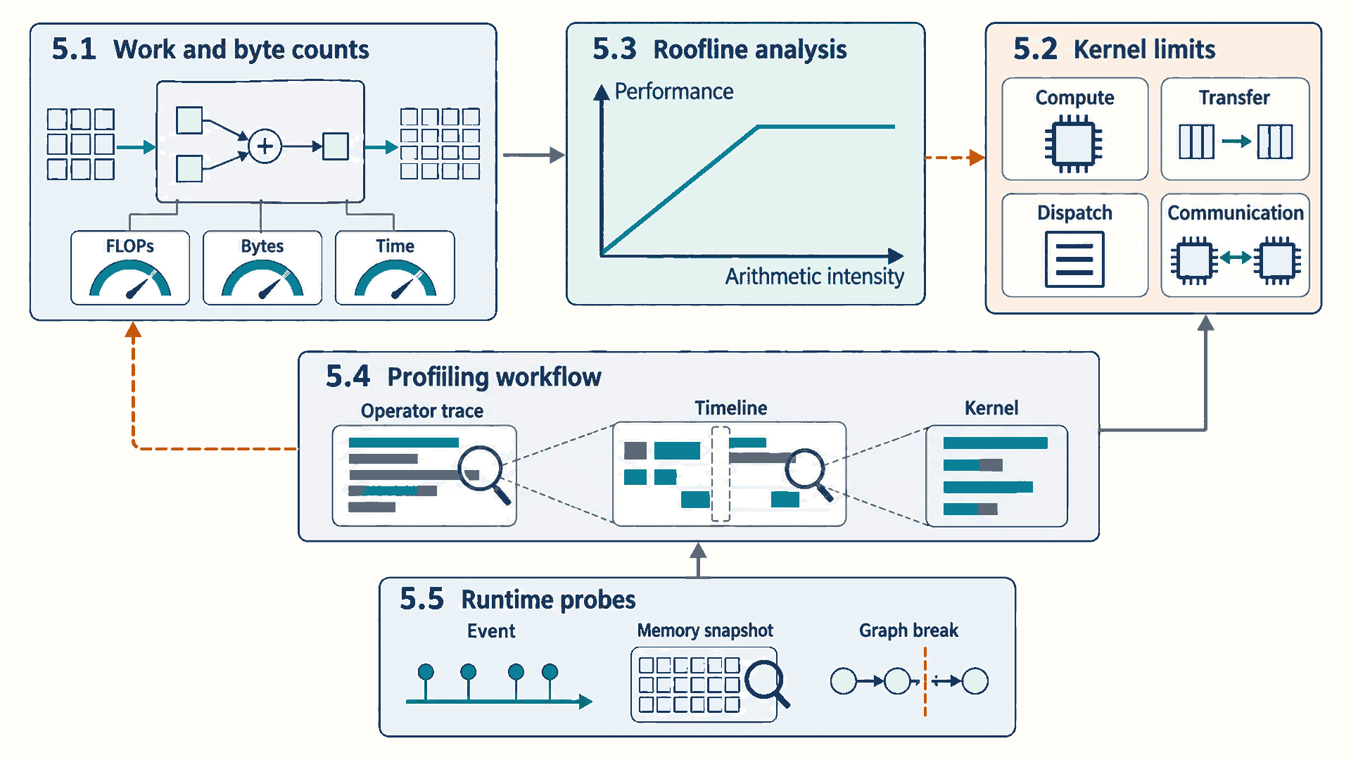
For an actual measurement, a point below a roof shows unused headroom but does not identify the cause by itself. The profiler timeline separately exposes launch gaps and other idle periods. A useful experiment changes one control that matches the measured symptom, then repeats the same measurement and correctness checks.

This chapter applies no lever. It decides which one applies: the roofline bound and the profiler timeline show whether a region is limited by arithmetic, by bytes, by too little parallel work, or by launch time, and Section 1.6.1 maps each of those limits to the levers that can move it.

5.1 Quantities and formulas

Performance models compare measured work, elapsed time, and data movement. The core quantities are floating-point operations, bytes moved through the memory level being modeled, arithmetic intensity, and achieved throughput. Section 2.8 introduced arithmetic intensity and the ridge point. This section fixes the counting rules they depend on, because both the roofline model and profiler results use them. Arithmetic intensity is written as:

\[ \text{AI} = \frac{\text{FLOPs}}{\text{bytes moved}} \tag{5.1}\]

The numerator and denominator must describe the same measured region and memory boundary. The definitions below make those counting choices explicit.

• AI: Arithmetic intensity, measured in FLOPs per byte. Higher AI means more arithmetic is performed for each byte moved.
• FLOPs: Floating-point operations performed by the kernel or phase. The count must match the operation being timed.
• bytes moved: Estimated traffic through the memory level being modeled, usually HBM for a first roofline pass. If the byte estimate ignores cache reuse or temporary buffers, the roofline conclusion can be wrong.

For example, 2e12 FLOPs and 1e12 bytes gives AI = 2 FLOPs/byte. The formula is useful because it forces an explicit byte estimate, but it omits cache effects, compression, metadata traffic, and hidden workspace movement.

Table 5.1: Byte-count starting points. They are lower bounds or first-pass estimates, not replacements for profiler counters.

Workload fragment	First byte-count estimate	What the estimate misses
Vector read and write	Read n elements and write n elements: about 2 x n x dtype_bytes	Cache reuse, write allocation policy, alignment, and vectorized transaction granularity.
GEMV y = Ax	Read M x N matrix values, read N vector values, and write M outputs	Repeated vector reuse from cache, partial sums in registers, batching, and fused epilogues.
GEMM C = AB	Read A and B and write C as a lower bound	Tiling can reuse A and B many times from on-chip storage, while poor tiling can add extra movement.
Naive attention scores	Materializing scores costs batch x heads x sequence x sequence x dtype_bytes for the score tensor alone	Masks, softmax temporaries, dropout, and whether an IO-aware kernel avoids the score tensor entirely.
KV-cache decode read	Read cached K and V for active tokens, layers, KV heads, head dimension, and dtype	Paged-cache metadata, cache locality, GQA/MQA head sharing, quantized cache formats, and batching policy.

The arithmetic count can be derived from the same dimensions as the byte estimate. In C = AB, with shapes (M, K), (K, N), and (M, N), there are M*N output entries. Each accumulates K products. Counting one multiply plus one add as two FLOPs gives the usual estimate 2*M*N*K, even when a fused multiply-add is one machine instruction¹. This convention counts accumulation from zero. A dot product written as K multiplies and K-1 additions has an exact algebraic count of 2*K-1 instead. Bias, activation, output scaling, and other final operations are additional work if they are inside the measured region. For Chapter 4’s GEMV, A has shape (M, N), so the same convention gives 2*M*N FLOPs.

Achieved throughput is computed from the measured runtime:

\[ \text{achieved throughput} = \frac{\text{FLOPs}}{\text{seconds}} \tag{5.2}\]

This quotient is valid only when the operation count and elapsed time cover the same work. Its three terms therefore need to be reported together.

• FLOPs: The same operation count used in the roofline estimate.
• seconds: Measured elapsed time for the same region. Include launch, synchronization, and communication only if those costs are part of the question.
• throughput: Measured work rate, usually reported as TFLOP/s for deep learning kernels.

If the same 2e12-FLOP kernel runs in 0.020 seconds, achieved throughput is 100 TFLOP/s. This is an illustrative rate calculation, not a reported measurement or a hardware property. It becomes misleading when warmup, compilation, or unrelated synchronization is included accidentally.

Achieved FLOP/s describes one kernel. A training run needs the same question answered for the whole model. Model FLOPs utilization (MFU) is the ratio of the arithmetic rate the model requires to the hardware’s peak rate: tokens processed per second times FLOPs per token, divided by the peak FLOP/s of the GPUs. For training, a rough dense-model estimate is \(6N_p\) FLOPs per token, using the projection-weight counting convention (Section 1.4), plus an attention term that grows with sequence length. MFU counts only the operations that forward and backward passes require, so activation-checkpointing recomputation is excluded from its operation count. Checkpointing can still change MFU by changing achieved tokens per second. Comparisons need the same model-work convention and matching dtype-specific hardware peaks.²

Worked example: MFU of a training run

Inputs: An 8B-parameter model trains across eight H100 SXM GPUs at an illustrative aggregate 64,000 tokens per second. Each GPU’s dense BF16 peak is about 989 TFLOP/s (Section 2.8). The 8B parameter count is used as the same rough projection-count proxy as in Section 1.4, and the attention term is ignored. This is an arithmetic example, not a measured run. The model and training state must be distributed with a per-GPU memory budget as described in Chapter 13.

Calculation: The model requires \(64{,}000\times6\times8\times10^9=3.072\times10^{15}\) FLOP/s. Dividing by the eight GPUs’ total peak, \(8\times9.89\times10^{14}=7.912\times10^{15}\) FLOP/s gives an MFU of about 39 percent.

Conclusion: MFU compares runs by the useful arithmetic they complete. The gap to peak does not identify a time breakdown. Memory-bound work, recomputation, communication, launch gaps, instruction mix, and idle time can all contribute. A profile is needed to distinguish them.

Monitoring tools report a different quantity under a similar name. The “GPU utilization” shown by nvidia-smi is the percentage of time over the sample period during which one or more kernels was executing on the GPU.³ A single small kernel running continuously reports 100 percent while it occupies a tiny fraction of the SMs and arithmetic units. That figure therefore detects idle gaps between kernels, but it cannot show how efficiently the GPU works while kernels run. MFU and the kernel metrics in Section 5.4.3 can.

A roofline estimate compares the compute ceiling with the bandwidth ceiling⁴:

\[ \text{roofline bound} = \min(\text{peak compute}, \text{AI} \times \text{peak bandwidth}) \tag{5.3}\]

The ridge point is the arithmetic intensity where the bandwidth ceiling reaches the compute ceiling:

\[ \text{AI}_{\text{ridge}} = \frac{\text{peak compute}}{\text{peak memory bandwidth}} \tag{5.4}\]

The two ceilings must refer to the selected dtype, operation path, and memory tier. These terms determine which side of the ridge point the workload occupies.

• peak compute: Best plausible arithmetic throughput for the selected precision, GPU generation, and kernel path. FP16, BF16, TF32 (NVIDIA’s reduced-precision mode for FP32 matrix math, Section 7.4), FP8, and integer formats have different ceilings.
• peak bandwidth: Relevant memory bandwidth for the modeled path. HBM bandwidth is not the same as NVLink, PCIe, or network bandwidth.
• AI times peak bandwidth: The bandwidth ceiling expressed as FLOP/s. It says how much compute can be sustained if every byte must be supplied at that bandwidth.
• ridge point: Arithmetic intensity at which the bandwidth ceiling and compute ceiling meet. Left of the ridge, bandwidth is the first-order limit. Right of the ridge, compute throughput is the first-order limit.

If AI = 2 FLOPs/byte and bandwidth is 3 TB/s, the memory ceiling is 6 TFLOP/s, so a 200 TFLOP/s compute peak does not matter for that kernel until reuse improves. The roofline omits scheduler overhead, launch overhead, synchronization, imperfect occupancy, dynamic shapes, and distributed communication.

Worked calculation: From matrix dimensions to a roofline bound

Inputs and work: Consider C = AB with M=64, N=32, and K=128, FP16 inputs and output, and no bias or read of an old C. There are 64*32 = 2,048 output entries, each with 128 multiply-add steps. At two FLOPs per step, the count is 2*64*32*128 = 524,288 FLOPs.

Bytes and intensity: Using the table’s one-read-per-input, one-write-per-output estimate gives 2*(64*128 + 128*32 + 64*32) = 28,672 bytes. FP16 occupies two bytes per stored value regardless of a wider accumulator. Arithmetic intensity is 524,288 / 28,672, approximately 18.29 FLOPs/byte.

Ceiling and interpretation: For illustrative matching ceilings of 200 TFLOP/s and 3 TB/s, the bandwidth roof is 18.29*3 = 54.86 TFLOP/s, below the compute roof. The model therefore predicts a bandwidth ceiling of about 54.86 TFLOP/s, not an achieved speed. The tiny shape can also be limited by launch overhead. Repeated HBM reads or extra writes increase the byte count and lower this roof, while inputs already in cache require a different HBM traffic estimate. No measured runtime is supplied for this calculation.

5.2 Limits on kernel performance

A measured region can take longer because it is moving bytes, performing arithmetic, waiting on dispatch, or waiting for other devices. The following labels make those causes explicit.

These categories are diagnostic, not labels for whole applications. One training step can contain compute-bound GEMMs, memory-bound optimizer updates, launch-bound small operations, and communication-bound gradient synchronization. The right optimization depends on the region being measured.

The following four labels describe a measured region. Each names the dominant cost and points to the first change worth testing:

• Memory-bound: Runtime follows bytes moved. Key-value cache reads during decode are a common example. Test locality, precision, coalescing, and cache layout.
• Compute-bound: Runtime follows arithmetic throughput. Large dense projections are a common example. Test Tensor Core use, dimension alignment, and useful batch size.
• Launch-bound: GPU work is short and CPU or dispatch gaps dominate. Many small eager operations are a common example. Test fusion, compilation, or CUDA Graph replay.
• Communication-bound: Collectives dominate the timeline. Distributed gradient synchronization is a common example. Test overlap, sharding, rank placement, and topology.

These four classes appear in local kernel traces and distributed training timelines. Section 1.6.1 lists the full set, including latency-bound, input-bound, capacity-bound, and scheduler-bound regions. Arithmetic intensity then tests whether memory bandwidth or compute throughput can explain the measured region.

5.3 Roofline analysis

A roofline derivation turns a measured or estimated kernel into a ceiling comparison. The input is FLOPs, bytes moved, elapsed time, peak compute, and memory bandwidth. The output is a first-order explanation of whether the kernel is plausibly limited by memory traffic or arithmetic throughput.

5.3.1 Constructing the model

The roofline chart places achieved throughput against arithmetic intensity on a log-log scale. Its diagonal memory-bandwidth ceiling and horizontal compute ceiling meet at the ridge point, which separates the first-order bandwidth-limited and compute-limited regions.

For one measured region, FLOPs divided by bytes moved place the point on the horizontal axis, while FLOPs divided by elapsed time place it on the vertical axis. The comparison uses bandwidth and compute ceilings for the same dtype, operation path, and memory level.

Figure 5.2: Roofline model

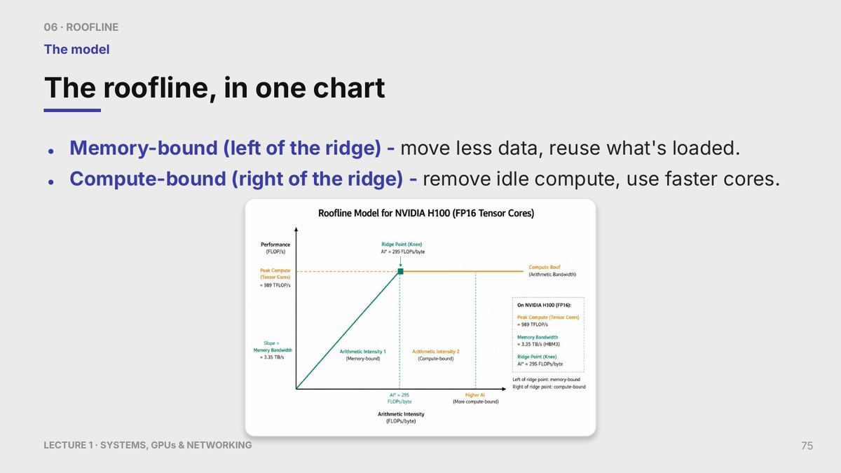
The printed ceilings are an H100 FP16 theoretical-peak example. In the first-order model, points left of the ridge are bounded by the memory roof and points right of it by the compute roof. A point below either roof still requires profiling before choosing a kernel, precision, or hardware change.

Chart note

Measured or compared: Achieved performance compared with hardware memory-bandwidth and compute-throughput ceilings.

Axes, units, and series: The horizontal axis is arithmetic intensity in FLOPs per byte. The vertical axis is performance or throughput. The diagonal series is the memory-bandwidth ceiling. The flat series is the peak-compute ceiling. The ridge marks where the active ceiling changes.

Interpretation: The bandwidth roof is lower to the left of the ridge, and the compute roof is lower to the right. Position alone does not establish the measured kernel’s bottleneck. A measured point far below the roof suggests locality, launch, synchronization, or counting problems.

Source status: The plotted values are not tabulated here. The surrounding equations provide worked numbers for reading the chart.

For a kernel with known FLOPs and estimated bytes moved, the arithmetic intensity places the kernel on the horizontal axis of the roofline chart. The achieved throughput places it on the vertical axis. Low arithmetic intensity means the bandwidth ceiling is low. High arithmetic intensity can move the kernel toward the compute ceiling. The ridge point is the diagnostic boundary: to the left, reduce bytes or increase reuse. To the right, improve arithmetic throughput, tensor-core utilization, or useful batch shape.

The derivation is deliberately approximate. If the measured point appears above the roofline, the FLOP count, byte estimate, measurement window, or peak numbers are inconsistent. That inconsistency is useful because it forces the engineer to refine the model before choosing an optimization.

Roofline limit

Peak compute and peak HBM bandwidth define an upper bound. Real kernels can sit below it because of instruction mix, occupancy limits, shared-memory bank conflicts, register spilling, Tensor Core alignment, synchronization, launch overhead, cache misses, or incomplete overlap. Profiler evidence explains the gap below the bound.

A point below the roofline shows unused headroom but does not identify whether launch gaps, occupancy, synchronization, or cache behavior caused it. The next question is whether a worked set of FLOPs, bytes, and elapsed time is internally consistent before an optimization is selected.

5.3.2 Worked roofline interpretation

A worked roofline pass counts FLOPs, estimates bytes moved, and measures runtime, then forms the two quantities below. The calculation that follows checks whether they are consistent with the hardware ceilings.

\[ \text{AI} = \frac{2 \times 10^{12} \text{ FLOPs}}{10^{12} \text{ bytes}} = 2 \text{ FLOPs/byte} \tag{5.5}\]

\[ \text{achieved throughput} = \frac{2 \times 10^{12} \text{ FLOPs}}{0.020 \text{ s}} = 100 \text{ TFLOP/s} \tag{5.6}\]

Worked calculation: Roofline diagnosis

Illustrative measurement record: Suppose the same region as in Section 5.1 has 2e12 FLOPs counted, 1e12 bytes estimated for that region, and 0.020 seconds recorded. The target GPU has a 3 TB/s peak-bandwidth estimate.

Arithmetic intensity: 2e12 / 1e12 = 2 FLOPs per byte.

Achieved throughput: 2e12 / 0.020 s = 100 TFLOP/s.

First-order ceiling: 2 FLOPs/byte x 3 TB/s = 6 TFLOP/s. The measured 100 TFLOP/s is above that ceiling, so the byte estimate, FLOP count, timing region, or assumed memory level must be wrong.

Next measurement: Profiler bytes, cache reuse, operation count, and timing boundaries identify the assumption that needs refinement before a kernel change is selected.

In LLM inference, this is why prefill and decode should not be tuned with one mental model. Large prefill projections are GEMM-like and can move toward the compute side of the roofline. Small-batch decode is often GEMV-like, repeatedly reading weights and key-value cache for few new tokens, so it tends to remain left of the ridge and bandwidth-sensitive unless batching or fusion changes the shape.

5.4 Profiling workflow

When the slow layer is not yet known, profiling connects a visible delay to the framework operation, kernel, copy, or host wait that produced it. PyTorch Profiler connects framework operations with CPU time, CUDA activity, shapes, and allocations⁵. Nsight Systems then reveals launch ordering and idle gaps⁶, while Nsight Compute applies after a specific kernel has been isolated⁷.

Worked example: PyTorch profiler pass

This profiling template measures CPU and CUDA activity for one warmed-up function. Warmup avoids mixing initialization or compilation with steady-state timing. cuda_time_total identifies GPU kernels and operations that dominate device time. profile_memory=True helps connect bottlenecks to allocation and tensor size. If CPU time dominates, kernel optimization alone may not help.

Code example: PyTorch profiler pass

import torch
from torch.profiler import profile, ProfilerActivity

device = torch.device("cuda", 0)
args = (torch.randn(1024, 1024, device=device),)

def fn(x):
    return torch.relu(x @ x)

for _ in range(5):
    fn(*args)  # warmup
torch.cuda.synchronize()

with profile(
    activities=[ProfilerActivity.CPU, ProfilerActivity.CUDA],
    record_shapes=True,
    profile_memory=True,
) as prof:
    fn(*args)

print(prof.key_averages().table(sort_by="cuda_time_total", row_limit=20))

This template runs several warmup iterations to initialize the PyTorch CUDA allocator and warm up the kernels before capturing execution. A torch.cuda.synchronize() call enforces the completion of warmup before the profiler’s active region begins. In the profile block, PyTorch logs operations, tensor shapes, and memory changes. The resulting printout sorts operations by CUDA execution time. Inspecting this table helps identify whether execution is dominated by slow GPU kernels, CPU-to-GPU memory copies, or allocator overhead.

5.4.1 Profiler selection

Different profilers answer different questions. Start with the cheapest tool that can disprove the current guess, then move to lower-level tools only when more detail is needed.

• Python profilers: cProfile deterministically records Python function calls and their timings, while py-spy periodically samples a running Python process with low intrusion. Both are useful for tokenization, request formatting, Python scheduling, and data-loader work, but they collect evidence differently.
• Event or tracing profiler: Records timed events and relationships. PyTorch Profiler links framework operations to CPU time, CUDA kernels, memory, and shapes⁸. Nsight Systems records a system timeline with CUDA launches, kernels, memory copies, NVTX ranges (named time spans that application code inserts into a trace), and collectives⁹.
• Kernel profiler: Inspects one GPU kernel in detail. Nsight Compute (NCU) reports occupancy, memory transactions, instruction mix, tensor-core usage, achieved bandwidth, and stall reasons¹⁰.
• Trace viewer: Perfetto (a browser-based trace viewer) or Chrome trace viewing helps inspect exported timelines interactively, especially repeated decode steps and CPU/GPU gaps.

Profiling adds overhead. It can change timing, perturb scheduling, and force extra synchronization. Treat profiled runs as diagnostic evidence, not final benchmark numbers. Once the bottleneck is identified, measure a clean steady-state run without heavy profiling instrumentation. Section 11.1 gives the full benchmarking procedure: warmup, fixed shapes, synchronized timing, correctness checks, and repeated samples.

The trace patterns below map onto the bottleneck classes of Section 1.6.1. Synchronization-bound and transfer-bound traces represent wait states that belong to the communication-bound or launch-bound classes, depending on what is waited for. A CPU/data-bound trace is input-bound or launch-bound.

• Compute-bound trace: Long GPU kernels with high arithmetic utilization, little idle gap, and evidence of tensor-core or math throughput limits.
• Memory-bound trace: Runtime tracks bytes moved. Kernels show high memory throughput but lower arithmetic utilization, often visible in decode or KV-cache-heavy paths.
• Synchronization-bound trace: CUDA synchronizations, blocking copies, or collectives create wait regions where useful GPU work cannot proceed.
• Transfer-bound trace: Host-to-device, device-to-host, or device-to-device copies occupy visible timeline spans and block the hot path.
• CPU/data-bound trace: GPU sits idle while the host handles tokenization, data loading, JSON parsing, sampling, or scheduler bookkeeping.
• Launch-bound trace: Many tiny kernels are separated by CPU launch gaps. Fusion, torch.compile, or CUDA Graphs may help if shapes and control flow are stable.

The first profiler should be the least expensive tool that can disprove the current bottleneck guess, and its instrumented timing should not be reported as clean benchmark performance. After selecting the tool, the next question is how one costly framework operation maps to the specific GPU kernel, copy, or host wait that produced its time.

5.4.2 From framework operation to kernel

A profiler must observe the layer where the suspected delay is created. Framework operations, system scheduling, individual kernel behavior, serving queues, and distributed transports require different evidence even when they appear in one end-to-end request.

The escalation path below starts with the application vocabulary and moves downward only when the current evidence isolates a narrower question.

Table 5.2: Profiler layers and the question each one can answer.

Question layer	Primary evidence	What it can establish	Next escalation
PyTorch operation	PyTorch Profiler	Expensive operations, dimensions, memory events, and the CPU/CUDA time split	Nsight Systems when timeline ordering is unclear
CPU/GPU timeline	Nsight Systems with NVTX ranges	Launch gaps, copies, synchronization, kernel order, and collective spans	Nsight Compute after one kernel is isolated
GPU kernel	Nsight Compute	Occupancy, transactions, cache sectors, instruction mix, tensor-core use, and stalls	Source or kernel rewrite guided by measured counters
Exported framework trace	Perfetto	Interactive inspection of repeated steps, ranges, and CPU/GPU gaps	Return to the profiler that records missing events

NVTX ranges supply application context to timeline tools. Label phases such as tokenization, prefill, decode, sampling, cache management, and communication so a kernel sequence can be connected to the request or training step that launched it.

Serving-engine metrics are developed in Chapter 10 because queueing and cache pressure belong to the serving control plane. NCCL logs and distributed traces are developed in Chapter 12 because transport selection depends on ranks and topology. With the responsible layer selected, the next question is how to read its symptom and confirm it with a second measurement.

5.4.3 Profiler symptoms

A profiler result is evidence from a trace or kernel report that points toward a bottleneck. It is not a final answer by itself. The same visible pattern can have several causes, so the useful workflow is to connect the result to the layer that produced it, then confirm with a second measurement.

• GPU gaps between kernels: The device timeline has idle spaces between short kernels. Common causes are CPU launch overhead, Python scheduling, implicit synchronization, data-dependent control flow, or a serving scheduler that cannot feed work fast enough. Confirm with Nsight Systems or a PyTorch Profiler timeline before rewriting kernels.
• High memory throughput with low math utilization: The kernel is likely memory-bound. The next question is which bytes dominate: HBM reads, cache misses, uncoalesced global loads, key-value cache reads, or host-device copies.
• Low occupancy: Too few warps are resident on each Streaming Multiprocessor (SM), or the kernel is limited by registers, shared memory, block size, or launch shape. Low occupancy is not always a bug. Some kernels are intentionally limited by another resource.
• Many tiny kernels: The workload may be launch-bound or suffering from graph fragmentation. First check whether fusion, torch.compile, or CUDA Graph replay can remove repeated host-side overhead.
• Long memory-copy spans: The trace is spending time moving data rather than computing. Distinguish CPU-to-GPU transfer, GPU-to-CPU transfer, peer-to-peer GPU transfer, and network transfer because each has a different fix.
• High cache-sector traffic: Nsight Compute may show that a kernel requests many L1 or L2 sectors for little useful payload¹¹. This usually points to poor coalescing, scattered strides, low spatial locality, or streaming data that is too large to reuse from cache. If sectors per request look reasonable but hit rate is still poor, check reuse distance, working-set size, and possible conflict patterns from stride or layout. Read counters by level: L1/TEX symptoms suggest per-SM access-pattern issues. L2 misses to device memory suggest HBM traffic. L2 misses to peer or system memory suggest remote or mapped-memory paths.
• Long collective spans: A distributed step may be communication-bound. Check whether ranks arrive late, whether NCCL used the expected fabric, and whether overlap with backward or layer computation is actually hiding the collective.
• Allocator spikes: Repeated allocation or fragmentation can appear as CPU overhead, device synchronization, or memory-pressure stalls. Reuse buffers, stabilize shapes, or inspect PyTorch allocator statistics before assuming the math kernel is slow.

Once a trace isolates one slow kernel, Nsight Compute separates its throughput ceiling, memory behavior, warp scheduling, launch shape, and source-level instruction cost¹². The table groups the report views by the question they answer.

Table 5.3: Kernel-level metric families. Exact counter names vary with GPU architecture and Nsight Compute version, so read them as categories first.

Nsight Compute view	What it answers	Example metric family to inspect
Speed of Light / SOL	How close the kernel is to compute and memory ceilings.	SM throughput, DRAM throughput, achieved occupancy, and roofline-like utilization summaries.
Memory Workload Analysis	Which memory level and transaction pattern dominate.	L1/TEX sectors, L2 hit rate, DRAM bytes, sector counts, and shared-memory table entries.
Scheduler and warp state	Why warps were not issuing instructions.	Warp stall reasons such as memory dependency, barrier, not selected, or execution dependency.
Launch statistics	Whether launch shape and resources limit parallelism.	Grid/block dimensions, registers per thread, shared memory per block, theoretical occupancy.
Source counters	Which source lines or instructions create the traffic.	PC sampling, instruction mix, tensor-core instructions, local-memory loads/stores from spills.

Profiler output is a map of hypotheses. A PyTorch table can say which operator is expensive, Nsight Systems can show whether the GPU is idle or communicating, and Nsight Compute can explain one kernel’s memory transactions and occupancy. Jumping directly from one table row to a rewrite is a common source of wasted optimization work.

5.4.4 End-to-end profiling case

The following illustrative protocol tests whether repeated host launch work slows a fixed decode workload. It specifies the evidence needed for a conclusion. It does not report a measured improvement.

Worked protocol: Testing a decode launch gap

Assumed workload: The proposed workload contains 32 requests, 512-token prompts, 64 generated tokens, one model revision, one GPU, and fixed sampling settings. The request arrival pattern, batch membership, and token counts remain the same in both runs. Early stopping is disabled for this fixed-token experiment, and token counts are checked after each run.

Input and state: Tokenization produces the fixed prompt IDs. Prefill builds the initial KV cache. Decode then appends one token per active request and reads the existing cache.

Evidence to collect: The launch-overhead hypothesis is worth testing if a baseline timeline shows short decode kernels separated by CPU launch gaps. Kernel reports can test whether individual kernels are close to a memory or compute ceiling. Neither observation alone proves that graph replay improves request latency.

Proposed intervention: After warmup, CUDA Graphs capture an eligible stable decode region, as developed in Chapter 6. Request admission and variable-length control remain outside capture. The comparison keeps model arithmetic and kernel selection fixed so a timing change can be connected to launch behavior.

Comparison record: Repeated baseline and replay runs without profiler instrumentation supply TPOT and 95th-percentile (p95) request latency, using the same timing boundaries. The record includes values, run-to-run spread, and the number of requests and repetitions. Separate diagnostic traces compare GPU idle gaps and kernel durations because profiling can change latency. Compile and capture time remain outside steady-state decode. Correctness checks compare logits within a declared dtype-appropriate tolerance and generated tokens under fixed deterministic selection before interpreting performance.

Conditional conclusion: Reduced launch gaps together with unchanged kernel work, passing correctness checks, and a repeatable TPOT reduction support a launch-overhead explanation. A p95 improvement supports a benefit to slower requests only if it exceeds the observed run-to-run variation. Smaller gaps without lower TPOT do not establish an end-to-end gain. Unchanged or worse p95 means tail latency has not improved. Persistent gaps call for further checks of CPU scheduling, batching, or cache management. This protocol supplies no before/after measurements, so no speedup is claimed.

5.5 Runtime API probes

A runtime API probe is a small code fragment that asks one narrow question about the execution layer. Probes like these check device capability, dtype footprint, GPU timing, trace export, and compiler graph breaks before applying larger optimizations.

The probe follows the current question. Device capability and dtype establish hardware ceilings or byte counts. CUDA events measure kernel timing. A profiler trace shows operation ordering and gaps. TorchDynamo diagnostics reveal a split compiled function. Additional probes are useful only when the first result leaves the cause unclear.

Worked example: Device capability and dtype footprint

This probe shows that torch.cuda owns device visibility and basic CUDA runtime facts, while a tensor’s dtype determines its byte footprint. get_device_capability is a hardware probe, not a guarantee that every desired kernel path is enabled. element_size connects dtype to memory traffic: one million BF16 values occupy about two megabytes before allocator overhead.

Code example: Device capability and dtype footprint

import torch

device = torch.device("cuda", 0)

print(torch.cuda.get_device_name(device))
print(torch.cuda.get_device_capability(device))

x = torch.empty(1_000_000, dtype=torch.bfloat16, device=device)
bytes_per_element = x.element_size()
footprint_bytes = x.numel() * bytes_per_element

print(bytes_per_element, "bytes per element")
print(footprint_bytes, "total bytes")

Worked example: CUDA event timing

This probe measures elapsed time on the CUDA stream rather than trusting an unsynchronized CPU timer. It places input allocation and warmup outside the measured region. The expression y = x @ w still creates an output tensor between the events, so this probe measures that operation’s stream interval rather than isolating arithmetic alone. CUDA launches are asynchronous from the CPU side, so CPU wall-clock timing can accidentally measure queueing rather than device execution. Events measure work between markers on a stream. They still need synchronization before reading elapsed time.

Code example: CUDA event timing

import torch

device = torch.device("cuda", 0)
x = torch.randn(4096, 4096, device=device, dtype=torch.float16)
w = torch.randn(4096, 4096, device=device, dtype=torch.float16)

for _ in range(5):
    _ = x @ w
torch.cuda.synchronize()

start = torch.cuda.Event(enable_timing=True)
end = torch.cuda.Event(enable_timing=True)

start.record()
y = x @ w
end.record()

torch.cuda.synchronize()
print(start.elapsed_time(end), "ms")

When GPU memory remains occupied after a step, a memory snapshot records the state of PyTorch’s CUDA memory allocator at that point. torch.cuda.memory_snapshot() supplies that state. The simpler torch.cuda.memory_allocated() counter reports memory occupied by tensors, while torch.cuda.memory_reserved() includes unused memory retained by the caching allocator.¹³ Comparing these counters at the same completed-step boundary helps distinguish live tensor storage from reserved capacity. High reserved memory alone does not establish a leak. The snapshot supports investigation of allocation patterns; it is not a kernel-timing trace or a measurement of all GPU allocations outside PyTorch’s allocator.

Worked example: Profiler trace export

This abbreviated probe records one forward call, normally prompt prefill. It expects an already loaded causal language model on one CUDA device, accepting input_ids and use_cache=True without an incoming cache. input_ids is a nonempty (batch, prompt_length) torch.long tensor on that device, with equal-length, unpadded prompts. Model weights use the model’s supported floating dtype. Models that require additional masks or position inputs need those supplied according to their interface.

Warmup and synchronization occur before the recorded call. The exported single_forward_trace.json shows that call’s operations, copies, and gaps. use_cache=True requests cache creation, but this listing discards the returned cache and does not record repeated decode. Section 11.2.8, Cached decode state shows the required continuation: retain prefill’s past_key_values, pass one selected token of shape (batch, 1) to each later call, and keep the returned updated cache. To investigate repeated decode, profiling must enclose those later calls. Prefill remains outside that region when the question concerns decode alone. The table is diagnostic evidence, not a clean end-to-end latency measurement.

Code example: Single-forward profiler trace export

import torch
from torch.profiler import profile, ProfilerActivity

# Requires the model and unpadded prompt IDs described above.
model.eval()
with torch.inference_mode():
    for _ in range(3):
        warmup_out = model(input_ids=input_ids, use_cache=True)
        del warmup_out
    torch.cuda.synchronize(input_ids.device)
    with profile(
        activities=[ProfilerActivity.CPU, ProfilerActivity.CUDA],
        record_shapes=True,
        profile_memory=True,
    ) as prof:
        out = model(input_ids=input_ids, use_cache=True)
    del out

print(prof.key_averages().table(sort_by="cuda_time_total", row_limit=20))
prof.export_chrome_trace("single_forward_trace.json")

Worked example: Graph-break diagnosis

This probe uses TorchDynamo diagnostics to show why a Python function cannot remain one compiled graph. torch._dynamo.explain is a private API whose behavior can change across PyTorch versions. The scalar .item() forces a host-side value and creates data-dependent Python control flow, so the compiler must break the graph. This tool diagnoses compiler behavior. Confirm any resulting change with steady-state workload measurements. The usual fix is to express the branch with tensor operations or keep the compiled region away from scalar Python decisions.

Code example: Graph-break diagnosis

import torch
from torch import _dynamo as dynamo

def bad_step(x):
    if x.sum().item() > 0:
        return x * 2
    return x - 2

report = dynamo.explain(bad_step)(torch.ones(8, device="cuda"))
print(report)

These probes deliberately stay small. A probe should answer one layer question, then the engineer can decide whether the next step belongs to CUDA timing, graph capture, profiler inspection, serving-engine metrics, or distributed communication.

The profiler now separates kernel limits from host-side launch gaps and repeated framework work. Chapter 6 uses that evidence to decide when graph compilation, generated kernels, CUDA Graph replay, or ordinary eager execution (running each PyTorch operation immediately, one at a time) is the appropriate local runtime path.

---

1. NVIDIA. (2023). Matrix Multiplication Background User’s Guide, section 2, Math and Memory Bounds (last updated 2023-02-01). Official guide. Supports the two-FLOP multiply-add convention and 2MN*K GEMM estimate. Limit: arithmetic counts omit output scaling and other final operations unless added explicitly. The chapter’s small-shape calculation and hardware ceilings are illustrative. This source is also used in Chapter 3.

2. Chowdhery, A., et al. (2022). PaLM: Scaling Language Modeling with Pathways. arXiv:2204.02311. Section 4.1 defines model FLOPs utilization as observed tokens per second relative to the theoretical maximum at peak FLOPs, counting only the forward and backward operations and not rematerialization. Appendix B gives 6N matmul FLOPs per token plus 6LH(2QT) for dense attention. Limit: the chapter’s aggregate 64,000 tokens/s on eight GPUs is an illustrative input, not a reported result.

3. NVIDIA. (n.d.). nvidia-smi documentation. https://docs.nvidia.com/deploy/nvidia-smi/index.html. Support: the Utilization GPU field is the percentage of time over the past sample period during which one or more kernels was executing on the GPU. The sample period ranges from 1 second to 1/6 second depending on the product. Limit: the field does not measure how much of each SM or arithmetic unit is in use.

4. Williams, S., Waterman, A., & Patterson, D. (2009). Roofline: An Insightful Visual Performance Model for Multicore Architectures. Communications of the ACM, 52(4), 65-76. https://doi.org/10.1145/1498765.1498785. Supports the ceiling form min(peak compute, operational intensity times peak bandwidth), the ridge point where the roofs meet, and the bound and bottleneck reading used in 5.1 and 5.3. Limit: the paper models DRAM traffic after cache filtering on multicore CPUs; the chapter applies the same first-order reading to GPU HBM as a teaching model and adds GPU specific gaps separately.

5. PyTorch. (2.14 documentation; page created Dec 18, 2020, last updated May 11, 2026). torch.profiler. https://docs.pytorch.org/docs/2.14/profiler.html. Supports that the profiler context manager collects CPU and CUDA activity, that record_shapes saves input shapes, that profile_memory tracks allocation, and that shape tracing adds overhead. Limit: API flags and CUPTI behavior can change by release; the chapter uses the stable option names only.

6. NVIDIA. (n.d.). Nsight Systems User Guide. https://docs.nvidia.com/nsight-systems/UserGuide/index.html. Supports that Nsight Systems records a system timeline with CUDA launches, kernels, memory copies, NVTX ranges, and collectives such as NCCL. Limit: trace options and driver requirements vary by tool version; exact event names should be confirmed in the installed guide.

7. NVIDIA. (n.d.). Nsight Compute Profiling Guide. https://docs.nvidia.com/nsight-compute/ProfilingGuide/index.html. Supports per-kernel inspection with launch statistics, memory workload analysis, scheduler and warp-state views, and source counters including sector, occupancy, and stall families. Limit: exact counter and view names vary by GPU architecture and tool version, as the chapter states.

8. PyTorch. (2.14 documentation; page created Dec 18, 2020, last updated May 11, 2026). torch.profiler. https://docs.pytorch.org/docs/2.14/profiler.html. Supports that the profiler context manager collects CPU and CUDA activity, that record_shapes saves input shapes, that profile_memory tracks allocation, and that shape tracing adds overhead. Limit: API flags and CUPTI behavior can change by release; the chapter uses the stable option names only.

9. NVIDIA. (n.d.). Nsight Systems User Guide. https://docs.nvidia.com/nsight-systems/UserGuide/index.html. Supports that Nsight Systems records a system timeline with CUDA launches, kernels, memory copies, NVTX ranges, and collectives such as NCCL. Limit: trace options and driver requirements vary by tool version; exact event names should be confirmed in the installed guide.

10. NVIDIA. (n.d.). Nsight Compute Profiling Guide. https://docs.nvidia.com/nsight-compute/ProfilingGuide/index.html. Supports per-kernel inspection with launch statistics, memory workload analysis, scheduler and warp-state views, and source counters including sector, occupancy, and stall families. Limit: exact counter and view names vary by GPU architecture and tool version, as the chapter states.

11. NVIDIA. (n.d.). Nsight Compute Profiling Guide. https://docs.nvidia.com/nsight-compute/ProfilingGuide/index.html. Supports per-kernel inspection with launch statistics, memory workload analysis, scheduler and warp-state views, and source counters including sector, occupancy, and stall families. Limit: exact counter and view names vary by GPU architecture and tool version, as the chapter states.

12. NVIDIA. (n.d.). Nsight Compute Profiling Guide. https://docs.nvidia.com/nsight-compute/ProfilingGuide/index.html. Supports per-kernel inspection with launch statistics, memory workload analysis, scheduler and warp-state views, and source counters including sector, occupancy, and stall families. Limit: exact counter and view names vary by GPU architecture and tool version, as the chapter states.

13. PyTorch. (2.14 documentation). CUDA semantics, Memory management. Allocator state and memory counters. Supports allocator snapshots and the distinction between tensor allocation and cached reserved memory. Comparing repeated step boundaries is a diagnostic use of those counters, not proof of a leak or a complete account of other libraries’ allocations.