8  Inference Workloads

Explain the inference software path, prefill and decode metrics, memory sizing, and compression choices that determine request capacity and latency.

The training chapter followed a workload that changes model parameters. Inference starts from a loaded parameter set that normally stays fixed during a request and repeatedly applies it, but it still creates live software and memory objects: token IDs, temporary activations, logits, sampler state, request metadata, and a key-value cache that grows with the context.

One request has two different GPU phases, prefill and decode (Section 8.2), and they stress different hardware resources. Their shapes, reuse, and user-visible latency metrics differ, so neither phase should be assigned a bottleneck before it is measured.

The tokenizer, checkpoint, model, and inference-mode interfaces define the single-request baseline. Prefill and decode then establish the service metrics needed to size static parameters, batch-dependent state, and KV-cache capacity. Model compression (Section 8.7) can shrink that byte budget, and the remaining budget determines which cache layouts and allocation policies are practical in Chapter 9.

Serving begins before the first GPU kernel: a request waits for admission, is tokenized, runs prompt prefill, and then enters a repeated one-token decode loop.

Figure 8.1: An inference request passes through admission, prefill, and repeated decode while memory state grows.

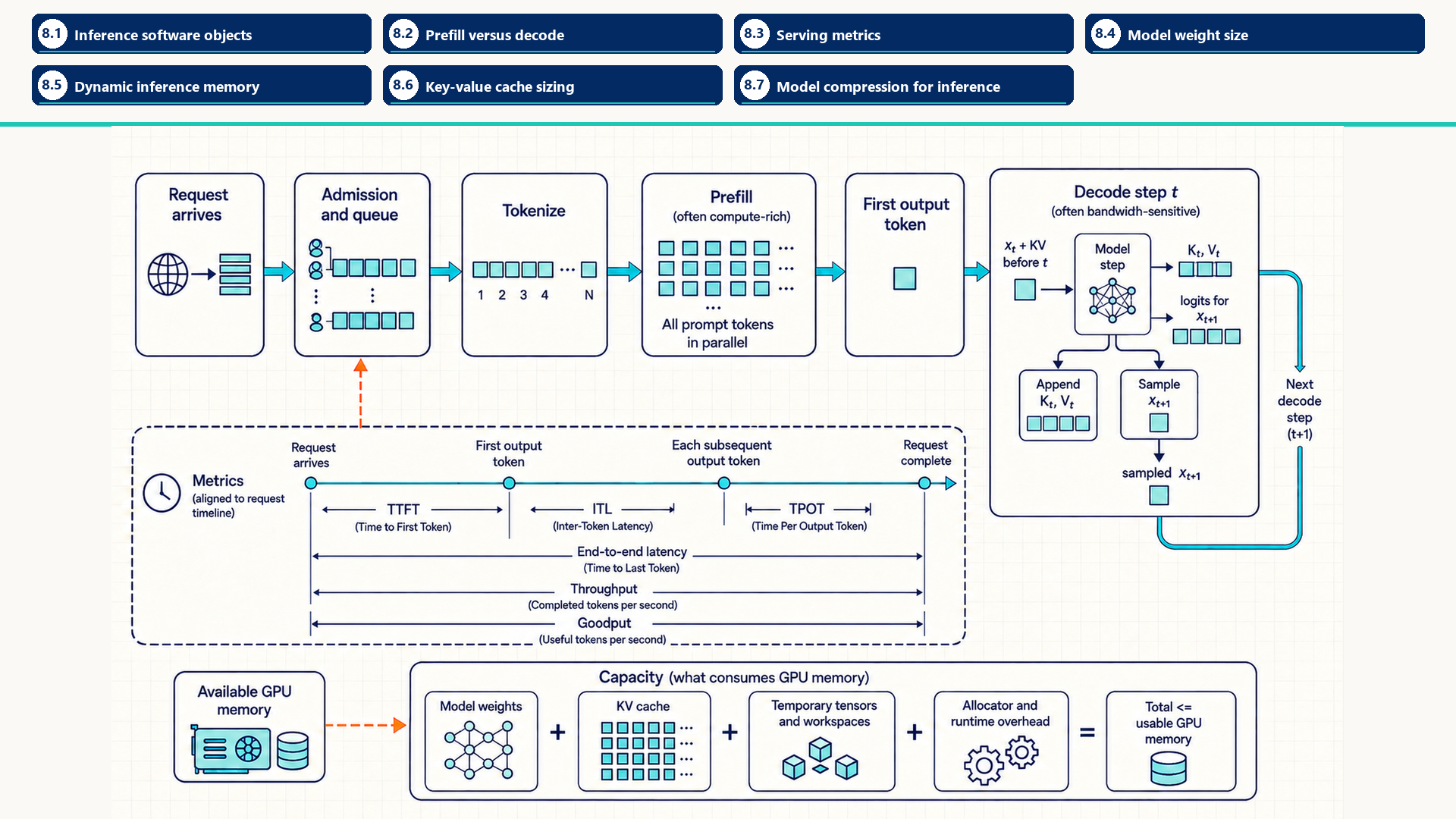
Each decode step reads the previous KV state, produces a new key and value pair plus logits, appends the new cache entry, and selects the next token. Time To First Token (TTFT), Inter-Token Latency (ITL), Time Per Output Token (TPOT), throughput, and goodput describe different parts of this path. The capacity budget must include weights, KV cache, temporary work, and allocator reserve.

The levers this chapter develops, in the vocabulary of Section 1.6.1, are do less work and move fewer bytes, through grouped-query attention and compression, and fit in memory, because weight and cache sizing decide what one GPU can hold.

8.1 Inference software objects

An inference request crosses several software objects before GPU kernels run. Tokenizer code creates token IDs, a model interface loads and executes the checkpoint, generation utilities control the baseline token loop, and a serving engine later adds shared scheduling and cache management.

8.1.1 Tokenizers and token-count effects

A tokenizer is the CPU-side software that maps text to token IDs and back. Its vocabulary, normalization, special-token policy, and segmentation algorithm determine the token count that drives prefill work, decode length, and KV-cache growth.

• AutoTokenizer: A Hugging Face Transformers factory that loads the tokenizer configuration associated with a checkpoint and returns a tokenizer object. Calling that object on text produces token IDs, masks, and batch encodings.
• SentencePiece: A tokenizer implementation family used by many model checkpoints. Its model file defines the segmentation and vocabulary used to create token IDs.
• Hugging Face Tokenizers: A high-performance tokenizer implementation used by many Transformers workflows for batching, truncation, padding, and special-token handling.
• Performance consequence: More prompt tokens increase prompt processing and initial KV-cache state even when the original character count is unchanged. Generated steps depend on the output tokens and stopping policy.

For a particular input and chat template, the tokenizer produces the input token IDs and fixes the prompt length. That length sets prefill work and the initial KV-cache size. The number of later decode steps depends instead on stopping criteria, requested output limits, and generation settings.

8.1.2 Model and checkpoint interfaces

A model interface creates the architecture and connects it to checkpoint tensors. Checkpoint loading determines storage format and startup behavior. Execution performance is later determined by placement, dtype, compiled or library kernels, and the serving runtime.

• AutoModelForCausalLM: A Hugging Face Transformers factory for autoregressive language-model architectures and checkpoints. It is useful for experiments, correctness checks, and baseline generation loops.
• safetensors: A tensor serialization format designed for safe, direct metadata inspection and efficient checkpoint loading. It owns storage and loading, not batching or kernel selection.
• Model configuration: The architecture metadata that defines layer count, hidden dimensions, attention heads, vocabulary, and other dimensions needed to construct the model before weights are loaded.
• Checkpoint tensors: Persistent parameter values loaded into CPU or GPU memory. Their format and placement affect startup and capacity, while the selected runtime path controls steady-state execution.

Separately, the model configuration defines the architecture and tensor shapes, while checkpoint loading places the stored parameters in memory.

8.1.3 Generation utilities and framework inference modes

Framework generation utilities provide a readable baseline token loop. PyTorch model mode and autograd mode must both be set correctly so inference uses evaluation behavior and avoids training-only bookkeeping. They do not by themselves make sampling or GPU execution deterministic.

• Generation utilities: Transformers helpers for cache-aware generation, sampling, beam search, stopping conditions, and token-loop control. They are convenient for experiments and baseline measurements.
• model.eval(): Changes module behavior such as dropout and batch-normalization statistics for evaluation or inference.
• torch.no_grad(): Disables gradient recording for enclosed operations, reducing autograd work and activation retention.
• torch.inference_mode(): A stricter inference context that also disables view tracking and version-counter updates for tensors created inside it.
• Combined use: Inference normally uses model.eval() with an appropriate gradient-disabling context. One controls module semantics. The other controls autograd bookkeeping.

These preparation paths meet when the application passes the token IDs to the loaded model. Evaluation mode controls module behavior, and an inference context disables gradient bookkeeping during the generation loop. Chapter 10 introduces a serving engine when many requests must share admission control (deciding which waiting requests may start), batching, KV-cache blocks, and operational metrics.

8.2 Prefill versus decode

Prefill and decode are two phases inside autoregressive inference serving. They use the same model weights, but they create different tensor shapes and stress different hardware resources. Separating them makes phase-specific measurement and optimization possible.

• Prefill: Processes the prompt tokens, computes attention over the input prefix, and writes the initial key-value cache. It creates persistent KV state for later decode steps as well as temporary work, and usually has many tokens available at once.
• Decode: Generates one new token per active sequence and appends new keys and values to the cache. It repeats many times and often has less arithmetic reuse per request.

The first comparison holds the model fixed and contrasts the two phases by input shape, likely limiting work, user metric, and available token parallelism.

Table 8.1: Prefill versus decode.

Dimension	Prefill	Decode
Input shape	Many prompt tokens	One new token per active sequence
Common limiting work	Projection and attention compute over the prompt; short prompts may still expose launch or scheduling cost	Weight and KV reads, launches, and scheduler delay; the dominant bytes depend on batch and context
User metric	TTFT	TPOT
Parallelism	High token parallelism	Low per-request parallelism, improved by batching

The arithmetic-intensity difference comes from reuse. During prefill, a batch contains many token positions, so projection weights and attention tiles can be reused across a larger matrix-shaped computation. During decode, each active sequence contributes only one new query token, while the step still reads model weights and a growing KV history. The same transformer block therefore behaves more GEMM-like in prefill and more GEMV-like or cache-streaming in small-batch decode.

Table 8.2: Prefill and decode arithmetic-intensity interpretation.

Phase	Reuse pattern	Arithmetic-intensity consequence	Capacity consequence
Prefill	Many prompt tokens reuse weights and attention tiles	Higher arithmetic intensity; tensor-core utilization is easier to recover	Long prompts increase TTFT and temporary activation/workspace pressure. They also create persistent KV-cache entries that affect admission and concurrency.
Decode	One new token reads weights and all relevant cached K/V state	Lower arithmetic intensity; HBM bandwidth, launch gaps, and scheduler overhead become visible	Long contexts and high concurrency mainly increase TPOT pressure and KV-cache capacity pressure
Continuous batching	Combines many one-token decode steps into a larger launched step	Improves useful work per launch but cannot remove serial dependence inside each sequence	Raises throughput until KV memory, latency targets, or scheduler cost becomes limiting

Because the two phases have different limits, FLOPs, bytes, and phase-specific latency are measured separately. A prefill optimization can improve TTFT while doing little for TPOT, and a decode optimization can increase throughput while consuming more KV-cache capacity.

The phase split now gives the first measurement boundary. TTFT describes the path through admission and prefill to the first generated token. TPOT and inter-token latency describe the repeated decode path.

8.3 Serving metrics

Inference metrics describe different stakeholders. A user notices the first token, the smoothness of streaming, and total completion time. An operator notices tokens per second, requests per second, GPU utilization, and cost. A Service-Level Objective (SLO) turns these into a measurable target, such as ‘95% of requests receive their first token within 500 ms.’ A Service-Level Agreement (SLA) is the contract that promises such a target to a customer. Engineering work optimizes against the SLO.

One-request timestamp trace

• A request-timing record includes request arrival, first-token emission, each later token emission, and completion.
• TTFT: Arrival to first-token emission.
• ITL: Each gap between consecutive output-token emissions.
• TPOT in this chapter: Excludes the first token and is the mean of the n - 1 decode intervals after first-token emission for a request with n > 1 output tokens. Other systems may aggregate TPOT differently, so those conventions require relabeling or recomputation before comparison.
• End-to-end latency: Arrival to completion.

Workload and operator metrics

• Report distributions of the chosen request-level measures, such as p50 and p95, without silently changing their aggregation convention.
• Throughput: Tokens or requests completed per second. State prompt length, output length, and workload mix.
• QPS, goodput, and cost: Must be tied to the SLO and quality target. Goodput counts only completed work that meets those targets.

\[ \text{E2E latency} \approx \text{TTFT} + (\text{number of output tokens} - 1) \times \text{TPOT} \tag{8.1}\]

In this approximation, the first output token is already included in TTFT. A response with n output tokens therefore contains n - 1 later decode intervals. TPOT is an average here. A production trace should also inspect the distribution of inter-token latency as batching, cache length, and scheduling change.

For example, if TTFT is 700 ms, the response has 20 output tokens, and average TPOT is 35 ms, then E2E latency is about 700 + 19 * 35 = 1365 ms. Long prompts mainly push TTFT because prefill must process many input tokens before streaming can begin. Long generations mainly push E2E latency through repeated decode steps. This is why the same optimization can improve one metric and harm another: larger batches can increase throughput and utilization while increasing queueing, TTFT, or ITL. These request times are also tied to concurrency: for a stable service, the average number of requests present equals the arrival rate times the average time each spends there. Cache residency depends on which of those requests have been admitted and retain KV state (Section 10.2.3).

8.4 Model weight size

Parameter sizing estimates the static model-weight footprint. It answers a different question from KV-cache sizing: weights are loaded once per replica or shard, while KV cache grows with active serving state. The estimate is useful for deciding whether a model fits on one GPU, one node, or a distributed group.

A transformer block is dominated by projection matrices. The formulas below are first-order approximations. Exact counts depend on vocabulary size, tied embeddings, grouped-query attention, bias terms, feed-forward expansion ratio, and architecture-specific details.

• Embeddings and language-model head: V * d parameters when the input embedding and output head share weights. An untied design contributes roughly 2 * V * d.
• Self-attention projection weights: about 4 * d^2 for standard full multi-head attention with d-by-d query, key, value, and output projections. Grouped-query and multi-query attention use smaller key/value projections.
• Multi-Layer Perceptron (MLP/FFN) Weights: about 8 × d² parameters. This consists of the up-projection (d-by-4d) and down-projection (4d-by-d). For models using SwiGLU activations such as Llama, the gate and up projections use a hidden size near 8/3 × d, so three matrices contribute about 3 × (8/3 × d²) = 8 × d² parameters¹. Adding bias terms adds comparatively little.

\[ \text{total parameters per block} \approx 12 d^2 \tag{8.2}\]

The symbols below define the estimate and the conversion from parameter count to stored bytes. They also mark what the block approximation leaves outside its boundary.

• V: Vocabulary size.
• d: Model hidden dimension.
• Block estimate: Approximate parameter count inside one transformer layer, excluding embedding and final output details unless stated.
• Memory conversion: Parameter count becomes bytes after multiplying by storage precision, such as 2 bytes for FP16/BF16 or fewer for supported quantized weights.

The local derivation is attention projections plus feed-forward projections: 4 × d² for Q, K, V, and output projection, plus about 8 × d² for the MLP, giving about 12 × d² per layer. With d = 4096, one block has about 12 × 4096² = 201,326,592 parameters. At 2 bytes per FP16/BF16 parameter, that block is about 402.7 MB before runtime workspaces, replica overhead, or quantization.

8.5 Dynamic inference memory

Batch shape is the actual tensor and scheduler shape admitted to the GPU. In LLM serving, a batch contains sequences with different prompt lengths, generated lengths, cache states, decode progress, and request count.

• Request batch size: The number of active requests. It is easy to count but insufficient for memory planning because one long request can consume more cache than many short requests.
• Tokens per iteration: The number of tokens actively processed in one forward pass (for example, all prompt tokens for new requests plus one token per decoding sequence).
• Tokens resident in KV cache: The total number of token positions retained across all active requests. Serving engines track both limits because one determines step time and the other determines memory capacity.
• Context length: The number of tokens a request can attend to. Longer contexts increase prefill work and KV-cache storage.
• Active cache blocks: Physical KV-cache blocks currently owned by admitted requests. This is the object that often limits concurrency.
• Prefill/decode mix: A batch can contain large prompt-processing work and one-token decode work. Mixing them improves utilization but can harm TTFT or inter-token latency if long prefill monopolizes the GPU.

Batch size improves hardware utilization only if memory can admit the active sequences. Sequence length and context length increase attention work and key-value cache size. A serving system therefore manages total batched tokens, cache blocks, the mix of prefill and decode work, and request count together.

8.6 Key-value cache sizing

Key-value cache sizing estimates the GPU memory consumed by stored attention keys and values for active requests. It is separate from model weight memory: weights are loaded once per replica, while the KV cache grows and shrinks with admitted sequences, context length, and generated tokens.

Section 1.3 introduced this estimate. It multiplies active sequences, stored tokens, layers, key and value tensors, head geometry, and dtype size:

\[ \text{KV bytes} = 2 \times B \times T \times L \times H_{\text{kv}} \times d_h \times b \tag{8.3}\]

The variables below identify the quantities in the estimate and connect each one to a serving decision.

• B: Active batch size or number of active sequences admitted by the serving scheduler.
• T: Sequence length stored in cache. This includes prompt tokens and generated tokens that remain in the attention context.
• L: Number of transformer layers that maintain KV state.
• 2: Two cached tensors per layer: keys and values.
• H with subscript kv: Number of key-value heads. This can be smaller than the number of query heads in grouped-query attention (GQA) or multi-query attention (MQA), which reduces cache size.
• d with subscript h: Head dimension for each key or value vector.
• b: Bytes per cached element, such as 2 bytes for FP16/BF16 or fewer bytes for supported KV-cache quantization (Section 8.7.1).

For example, B = 16, T = 4096, L = 32, key-value heads = 8, head dimension = 128, and 2-byte elements use 8,589,934,592 bytes: about 8.59 GB decimal or exactly 8 GiB. This is dynamic serving state, not model weight memory. This raw-payload estimate assumes equal retained lengths, the same KV geometry in every layer, and no cross-request prefix sharing. Unequal lengths require a sum over requests, and mixed layer layouts require a sum over layers. Shared prefixes are counted once per physical copy. Fragmentation, padding, metadata, and workspaces add overhead to the resulting payload.

Worked real-scale example: Llama 3.3 70B

Example configuration: Use 80 transformer layers, 8 key-value heads, head dimension 128, one active sequence, 32,000 cached tokens, and BF16 storage at 2 bytes per element²³.

Substitution: The formula gives 1 x 32,000 x 80 x 2 x 8 x 128 x 2 = 10,485,760,000 bytes.

Calculated size: That is about 9.77 GiB for one sequence before block-table metadata, allocator fragmentation, scales, workspaces, and other live tensors. If 32K means 32,768 tokens rather than 32,000, the same calculation is exactly 10.00 GiB.

Serving consequence: A single long-context request can consume a material fraction of an 80-GB GPU even when the model weights are already resident. Concurrency planning must budget KV cache separately from weights.

Multi-head attention variants change the key-value head count in that formula. Query heads decide how many independent query projections are used for the current token. Key-value heads decide how many historical key and value streams must be stored and reread. GQA and MQA reduce cache memory because several query heads share fewer key-value heads⁴⁵. The table holds layer count, head dimension, retained tokens, batch size, and cache dtype fixed, so it isolates the effect of the query-to-KV head ratio.

Table 8.3: MHA, GQA, and MQA cache multipliers.

Attention form	Head relationship	KV-cache multiplier versus full MHA	Serving consequence
MHA	Each query head has its own key and value head	1.0	Highest KV-cache footprint; simplest mental model
GQA	Groups of query heads share fewer key and value heads	key-value head count divided by query head count	Retains more independent KV head groups than MQA; quality and kernel behavior still require measurement
MQA	All query heads share one key and value head	1 divided by query head count	Smallest KV-cache footprint, but architecture quality and kernel support must be validated

For a concrete GQA example, a 32-query-head model with 8 key-value heads stores one quarter as many KV head streams as full MHA: 8 divided by 32 is 0.25⁶. If the same cache is also stored in 8-bit form instead of FP16/BF16, the raw element bytes are halved again before scale metadata (the stored scale factors, Section 8.7.1) and padding are added.

Table 8.4: KV-cache dtype byte multipliers.

KV-cache element format	Raw bytes per value	Multiplier versus FP16/BF16	Caveat
FP16 or BF16	2	1.0	Common baseline for cache sizing
FP8 or INT8	1	0.5 before scale metadata	Needs attention kernels and cache layout that support the format efficiently
INT4	0.5	0.25 before scale metadata	Can be attractive for capacity, but dequantization cost and attention quality are higher risk

8.7 Model compression for inference

Sections 8.4 and 8.6 sized the bytes an inference step must hold and read: the weights at every step, and the KV cache for every active token. Section 2.8 showed why a small decode step can be limited by moving those bytes. Model compression reduces them. Its four families differ in what they change and in what they cost:

Table 8.5: The four model-compression families compared.

Family	What changes	Main saving	Main cost	Section
Quantization	The number format of stored weights, activations, or KV cache	Fewer bytes per value	Rounding error, and the kernels must read the compact format	Section 8.7.1 to Section 8.7.4
Pruning and sparsity	Selected weights become zero and are skipped	Fewer stored weights, and fewer multiplications when the hardware supports the pattern	Accuracy loss, and a speedup only for supported sparsity patterns	Section 8.7.5
Distillation	A smaller model is trained to imitate a larger one	Fewer parameters in total	A separate training run, and the result is a different model	Section 8.7.6
Architectural reduction	The model is designed to store less state, as with grouped-query or sliding-window attention	A smaller KV cache	Requires a compatible architecture, training or adaptation	Section 8.6, Section 9.7

A smaller representation improves execution only when the runtime reduces the limiting work or memory traffic, or admits useful work that previously did not fit. Low-bit kernels may dequantize values inside the computation without materializing a full wider tensor. Expanding a compact checkpoint into full 16-bit tensors before each matrix multiplication can erase the traffic saving, so file size alone does not establish a speedup. Every family can change the model’s outputs, so each needs a quality check on the intended workload (Section 8.7.4).

8.7.1 Deployment quantization

Deployment quantization starts with an already-trained model and changes how selected tensors are represented at inference time. It is useful when the measured bottleneck is weight or cache bytes, memory capacity, or a hardware path that efficiently consumes the compact representation.

• Weight quantization: Stores model parameters in fewer bits. It mainly targets persistent weight memory and repeated weight reads during inference.
• Activation quantization: Stores or computes intermediate tensors in lower precision. It can reduce traffic between operations, but it is more sensitive to calibration because activation distributions vary with data.
• KV-cache quantization: Stores attention keys and values in fewer bits during serving. It targets the dynamic memory object that grows with active requests and context length.
• Dequantization: Conversion from a compact representation back to a wider representation for computation. If dequantization is expensive or happens too early, the latency benefit can disappear.
• Scale metadata: Extra values that map low-precision integers or floating formats back to approximate real values. Group size and scale placement affect both quality and kernel cost.

Affine integer quantization stores an integer code \(q\) for a real value \(x\). The positive scale \(s\) sets the size of a quantization step. The integer zero point \(z\) is the code that represents the real value zero. Clipping limits the code to the target format’s range \([q_{\min},q_{\max}]\), for example \([-128,127]\) for a signed 8-bit integer. The runtime later reconstructs an approximate wider value when a kernel needs it:

\[ q = \text{clip}\left(\text{round}\left(\frac{x}{s}\right) + z, q_{min}, q_{max}\right) \tag{8.4}\]

\[ \text{dequantized } x = s \times (q - z) \tag{8.5}\]

The numerical trace in Section 8.7.4 follows observed values through scale selection, rounding, clipping, and reconstruction using these two mappings.

The stored code is smaller, but the end-to-end gain depends on where the second mapping occurs. A fused low-bit matrix kernel can unpack codes, apply scales, and accumulate without first materializing a full FP16 or BF16 tensor. A separate early dequantization pass can give back much of the saved memory traffic.

When a workload is memory-bound (Section 2.8), reducing bytes moved can be more valuable than reducing arithmetic. Evaluate whether the hot path avoids reading, writing, or transferring the wider representation.

8.7.2 Quantization methods

Quantization can target three different tensor families, and each family belongs to a different part of the execution path. Weights are persistent model parameters read by linear layers. Activations are intermediate values produced while executing a request or training step. The key-value cache is serving-time attention state stored across decode steps. Each family requires compatible formats, kernels, scaling metadata, and quality validation.

Weight-only quantization is usually the simplest inference path: it shrinks parameters while leaving activations in a higher precision. Activation quantization is more intrusive because activation distributions vary by layer, token, and workload. Key-value cache quantization targets long-context serving capacity and decode bandwidth, but it can affect attention quality and needs engine support.

• GPTQ: A post-training weight quantization method that uses approximate second-order information to choose quantized weights with lower reconstruction error than naive rounding⁷. It is commonly used for low-bit inference checkpoints when compatible kernels exist.
• AWQ: Activation-aware Weight Quantization. It protects weight channels that are important for activations drawn from the expected workload, reducing quality loss for low-bit weight-only inference⁸.
• FP8 and KV-cache quantization: FP8 targets lower-precision tensor and cache storage with hardware/runtime support. KV-cache quantization reduces long-context memory pressure but can introduce dequantization cost and attention-quality risk.

AWQ and GPTQ are method families, not runtime guarantees. Their checkpoints reduce weight bandwidth only through the kernel paths described in Section 8.7.3.

Table 8.6: Quantization methods as performance techniques.

Method	Mechanism	What it helps	What still must be checked
GPTQ	Uses calibration data and approximate second-order reconstruction to choose low-bit weights with lower layer-output error than naive rounding	Weight-only low-bit inference when parameter reads or model fit are the bottleneck	Quantization time, compatible kernels, quality on prompts from the expected workload, and whether dequantization stays fused
AWQ	Uses calibration activations from the expected workload to find important channels and protects them through activation-aware scaling before low-bit weight quantization	Hardware-friendly weight-only inference where a small set of important channels drives error	Calibration domain, packed-weight layout, kernel support, and whether activation outliers shift in production
FP8 path	Stores or computes selected tensors in FP8 with scaling factors and wider accumulation where required	Bandwidth, tensor-core throughput, activation or KV-cache footprint on supported accelerators	Scaling granularity, amax handling, supported operations, and numerical quality

8.7.3 Quantization libraries and kernel support

A quantization method becomes a runnable performance path through a library and compatible kernels. The implementation owns packing, scale metadata, conversion, supported devices, and the operations that can consume the compact representation.

• bitsandbytes: A low-precision training and inference library with quantized optimizer and weight paths⁹. Its benefit depends on the selected model, format, GPU, and kernel support.
• torchao: PyTorch-native quantization and sparsity tooling that integrates supported low-precision representations with PyTorch models and execution paths¹⁰.
• Implementation support: The concrete combination of packed layout, scale granularity, dequantization strategy, matrix kernel, GPU architecture, and runtime version that turns a small checkpoint into a fast execution path.
• Measurement boundary: Checkpoint size demonstrates storage compression. End-to-end latency, throughput, peak memory, and quality demonstrate whether the implementation helps the workload.

Library names serve as implementation examples rather than definitions of quantization. GPTQ, AWQ, FP8, INT8, and INT4 describe methods or formats. Bitsandbytes and torchao provide selected software paths for them.

8.7.4 Calibration, PTQ and QAT

Calibration chooses quantization parameters from tensors drawn from the expected workload. Hardware support determines whether the GPU and runtime have fast kernels for the chosen format. Offline calibration is needed by static activation quantization and methods such as GPTQ or AWQ. Dynamic activation quantization derives ranges during execution, and some weight-only methods use weight statistics without a separate workload calibration run¹¹.

• Calibration set: Prompts, activations, or layer inputs drawn from the expected workload and used to estimate value ranges.
• Scale: A multiplier that maps low-precision stored values back to approximate real values. Scales can be per tensor, per channel, per group, or more specialized depending on the method.
• Clipping range: A selected numeric range that limits outliers before quantization. Aggressive clipping can improve average reconstruction but harm rare important values.
• Per-channel or per-group quantization: Uses separate scales for smaller tensor groups. This usually improves quality relative to one global scale, but increases metadata and kernel complexity.
• Weight-only calibration: Focuses on parameter tensors and workload-derived activations used by methods such as GPTQ or AWQ.
• Activation and KV-cache calibration: Targets runtime tensors whose distributions depend on prompts, sequence length, layer, and model behavior. Mistakes here can produce quality loss that a simple file-size check does not reveal.

Two deployment paths differ in when low-precision behavior enters the model lifecycle. The third entry is the gradient approximation that the second path depends on:

• Post-Training Quantization (PTQ): Converts an already-trained model for lower-precision deployment. For a calibrated static path, a run records weight or activation ranges from the expected workload, derives scales and zero points, and packs the selected tensors. Dynamic and weight-only paths can obtain their parameters differently. All paths need quality and runtime checks.
• Quantization-Aware Training (QAT): Trains with fake quantization and dequantization operations in the forward pass, so model updates see an approximation of the error introduced by the deployed representation.
• Straight-Through Estimator (STE): A backward-pass approximation used for a rounding-like fake-quantization operation. It substitutes a usable derivative estimate so gradient-based optimization can continue.

Worked example: From calibration values to integer codes

Inputs and policy: A toy inference activation tensor supplies calibration values \([-2,-0.6,0,1.4,5]\). To expose the arithmetic, allow just eight integer codes, \(q_{\min}=0\) through \(q_{\max}=7\). This is a teaching code range, not a claim about a deployed three-bit kernel. Apply the affine min/max policy documented by PyTorch’s MinMaxObserver: \(s=(x_{\max}-x_{\min})/(q_{\max}-q_{\min})\) and \(z=q_{\min}-\operatorname{round}(x_{\min}/s)\)¹². The observed interval already includes zero. Round to nearest, with halfway ties going to the even integer, then clip the code to \([0,7]\) and reconstruct \(\hat x=s(q-z)\)¹³.

Calibration: The observed minimum is \(-2\) and maximum is \(5\), so \(s=(5-(-2))/(7-0)=1\) and \(z=0-\operatorname{round}(-2/1)=2\). Zero therefore receives code \(2\). The last row below adds a later value of \(12\) while keeping the calibrated scale fixed. Signed error means \(\hat x-x\).

Table 8.7: Quantization of calibration values with the scale held fixed.

Input \(x\)	\(x/s\)	Rounded value plus \(z\)	Clipped code \(q\)	Reconstruction \(\hat x\)	Error
\(-2\)	\(-2\)	\(0\)	\(0\)	\(-2\)	\(0\)
\(-0.6\)	\(-0.6\)	\(1\)	\(1\)	\(-1\)	\(-0.4\)
\(0\)	\(0\)	\(2\)	\(2\)	\(0\)	\(0\)
\(1.4\)	\(1.4\)	\(3\)	\(3\)	\(1\)	\(-0.4\)
\(5\)	\(5\)	\(7\)	\(7\)	\(5\)	\(0\)
\(12\)	\(12\)	\(14\)	\(7\)	\(5\)	\(-7\)

Outlier trade-off: Recalibrating with \(12\) included expands the interval to \([-2,12]\), giving \(s=14/7=2\) and \(z=0-\operatorname{round}(-1)=1\). The outlier now reconstructs exactly: code \(7\) gives \(2(7-1)=12\). But \(-0.6\) now reconstructs as \(0\) and \(1.4\) as \(2\), with errors \(+0.6\) in both cases. The former endpoint \(5\) maps through \(5/2=2.5\), rounded to \(2\), to code \(3\) and reconstruction \(4\). Accommodating the outlier doubled the step size for every value sharing this scale.

Conclusion: Keeping the original range preserves finer spacing but clips the outlier. Expanding it protects the outlier while increasing some smaller-value errors. Separate groups can fit different ranges at the cost of more scale metadata and kernel work. These arithmetic errors do not determine task quality by themselves. This example implements neither GPTQ nor AWQ, FP8 scaling, or every PTQ calibration recipe.

During QAT, the forward pass applies \(\operatorname{fake\_quant}(x)\), a simulation of the chosen deployment quantization. Rounding has zero derivative between its jumps and is not differentiable at the jumps, so its true derivative cannot provide the usual learning signal. A clipped STE instead passes the incoming gradient through inside a chosen representable interval and blocks it outside. For the affine mapping above, use \(x_{\min}=s(q_{\min}-z)\) and \(x_{\max}=s(q_{\max}-z)\). The following is a backward approximation, not the true derivative of quantization. Implementations may differ at the clipping boundaries:

\[ \text{STE backward rule: } \frac{\partial \text{fake-quant}(x)}{\partial x} = 1 \text{ if } x \in [x_{min}, x_{max}] \text{ else } 0 \tag{8.6}\]

Here ∂ fake_quant(x) / ∂x means the rate of change assigned to the fake-quantization operator with respect to its input x. The equality defines the surrogate gradient used by backward propagation. It does not claim that the true derivative of rounding is one.

Calibrated PTQ adds an offline calibration step and may lose quality at low bit widths. QAT spends training compute to adapt the model to the deployed representation. Compare quality on requests drawn from the expected workload, then measure whether the selected engine uses the packed format in its hot kernels.

Quality is measured on the task, not on the tensors. Three checks are common, and each detects a different kind of damage. Perplexity (the exponential of the average per-token cross-entropy loss on held-out text, where lower is better) detects broad damage to the model’s predictions cheaply. Task accuracy on a fixed evaluation set, such as a public benchmark or a sample of production prompts with reference answers, detects damage that a small perplexity change can hide. A side-by-side comparison with the uncompressed model on the same prompts under greedy decoding shows how often, and where, the generated tokens diverge. The original and compressed models use the same prompts, tokenizer, and decoding settings, so that a difference can be attributed to the compression.

Group size is the local granularity of a quantization scale. It is one of the clearest examples of a performance-quality trade-off: the smaller the group, the better the scale can fit local values, but the more scale metadata and indexing work the kernel must carry.

Table 8.8: Group quantization trade-offs.

Group-size choice	Quality effect	Runtime effect	When it is attractive
Small groups	Better local reconstruction because fewer unrelated values share one scale	More scale reads, more metadata, and more complex packing or dequantization	Accuracy is fragile and kernels are designed for that grouping
Large groups	More values share a scale, so outliers can waste quantization range	Less metadata and simpler memory access	Bandwidth or metadata overhead dominates and quality remains acceptable
Per-channel groups	Fits channel-level activation or weight ranges	Works well when kernels can load scales along the channel dimension efficiently	Linear layers where channel statistics are stable enough under calibration
Per-block groups	Fits local blocks rather than whole tensors	Can align with tile layouts, but only if the backend expects that layout	FP8 or INT4 paths with block-scaled kernels

Poor calibration can preserve speed while harming quality. Poor hardware or kernel support can preserve quality while failing to improve latency.

8.7.5 Pruning and structured sparsity

Quantization keeps every weight but stores it in fewer bits. Pruning instead removes weights: it sets a chosen subset to zero so that they need not be stored or multiplied. Whether the zeros save time depends on where they fall, because GPU matrix kernels process regular tiles and gain nothing from zeros they cannot skip.

• Unstructured sparsity: any individual weights may be zero. It allows more freedom to choose which weights to remove than a fixed structured pattern, but accuracy depends on the pruning method and model. Dense GPU kernels cannot skip scattered zeros. The saving then requires a compressed storage format and specialized sparse kernels.
• Structured sparsity: whole rows, columns, attention heads, or blocks are removed. Removing complete channels or heads can produce smaller dense matrices after dependent tensors are resized. Removing isolated blocks instead needs a compatible block-sparse kernel. The quality cost depends on which structures are removed and any later adaptation.
• Semi-structured 2:4 sparsity: in every group of four consecutive weights, at most two are nonzero. The compressed format stores the two kept values plus a 2-bit position index for each, and the Sparse Tensor Cores of NVIDIA Ampere and later GPUs use it to double the math throughput of the dense units.¹⁴

Retraining a model with billions of parameters after pruning is expensive, so the methods below prune once, after training. SparseGPT prunes GPT-family models to at least 50 percent unstructured sparsity in one pass without retraining, reaches 60 percent on its largest models with a small perplexity increase, and extends to 2:4 and 4:8 patterns.¹⁵ Wanda removes the weights with the smallest magnitude multiplied by the L2 norm of the corresponding input feature across calibration tokens, comparing weights within each output row, also without retraining or weight updates, and is evaluated for unstructured, 4:8, and 2:4 sparsity.¹⁶

Worked example: What 2:4 sparsity saves in one projection

Inputs: The \(4{,}096\times4{,}096\) BF16 projection of Section 2.8, whose dense weights occupy \(2\times16{,}777{,}216=33{,}554{,}432\) bytes, is pruned to the 2:4 pattern.

Storage: Half the weights remain: \(8{,}388{,}608\) values at 2 bytes, or \(16{,}777{,}216\) bytes. Each kept value adds 2 bits of position metadata, \(8{,}388{,}608\times2/8=2{,}097{,}152\) bytes. The total is \(18{,}874{,}368\) bytes, 56 percent of the dense size.

Time: For one row, the bandwidth-only model gives a time floor of about \(18.9\text{ MB}/3.35\text{ TB/s}\approx5.6\) microseconds instead of 10.0, a 1.8-times ratio between these ideal floors. For a large batch that saturates compatible Sparse Tensor Cores, the doubled math peak permits an ideal 2-times arithmetic gain. Neither ratio predicts measured latency, which also includes kernel efficiency and overhead.

Conclusion: In the memory-bound regime 2:4 sparsity helps the way quantization does, by moving fewer bytes. In the compute-bound regime it helps by skipping multiplications. Both gains require a kernel that reads the 2:4 format, and both come after half of the weights have been removed, so model quality must be measured as in Section 8.7.4.

8.7.6 Distillation

Quantization and pruning shrink an existing model. Knowledge distillation trains a different, smaller one. A small student model is trained to reproduce the output distribution of a larger teacher model. Hinton et al. train on the teacher’s class probabilities, softened by raising the softmax temperature, as soft targets, and use the same temperature for the student.¹⁷ For a language model the targets are the teacher’s next-token distributions at each position, which carry more information per example than the single correct token.

The student’s serving cost follows its own size. An 8B student of a 70B teacher needs about \(2\times8\times10^9=16\) GFLOP per generated token instead of 140 GFLOP (Section 1.4), and reads 16 GB of BF16 weights per decode step instead of 140 GB, 8.75 times less. When teacher distributions are computed on demand during student training, each training token needs a teacher forward pass (\(2\times70\times10^9=140\) GFLOP) as well as the student’s forward and backward passes (\(6\times8\times10^9=48\) GFLOP), about 3.9 times the arithmetic of training the student alone on the same tokens. Precomputing teacher targets can amortize repeated teacher passes, at the cost of storing and reading those targets. These estimates count dense parameter arithmetic and omit attention-score work and runtime overhead.

Unlike quantization, distillation cannot be adjusted at deployment time. The student is a new model with its own quality profile, so it is evaluated on the target tasks like any other model. A distilled student can also serve as the draft model for speculative decoding (Section 10.6), where its agreement with the teacher sets the acceptance rate.

Sections 8.4 to 8.7 answer how many bytes a planned set of requests needs and how compression can reduce them. They do not say where each request’s state should be placed or how attention kernels find it. Chapter 9 turns this capacity estimate into a layout problem: token order must remain logical even when physical blocks are allocated, reused, and read non-contiguously.

---

1. Shazeer, N. (2020). GLU Variants Improve Transformer. arXiv:2002.05202. https://arxiv.org/abs/2002.05202. Supports the three matrix SwiGLU feedforward form and reducing hidden width to two thirds of the original width to match two matrix parameter count. Limit: the chapter uses near 8/3 times d as a coarse sizing convention; exact widths vary by model.

2. Meta Llama. (llama-models at commit 0e0b8c5, Oct 10, 2025). models/sku_list.py. https://github.com/meta-llama/llama-models/blob/0e0b8c519242d5833d8c11bffc1232b77ad7f301/models/sku_list.py. Supports Llama 3.3 70B Instruct with dim 8192, 80 layers, 64 query heads, 8 KV heads, and head dimension 128 from 8192 divided by 64. Limit: the worked numbers are a stipulated teaching example and exclude metadata, fragmentation, and workspace overhead.

3. Meta Llama. (llama-models at commit 0e0b8c5, Oct 10, 2025). models/llama3_3/MODEL_CARD.md. https://github.com/meta-llama/llama-models/blob/0e0b8c519242d5833d8c11bffc1232b77ad7f301/models/llama3_3/MODEL_CARD.md. Supports that all Llama 3.3 versions use grouped-query attention for inference scalability, with the 70B Instruct release dated December 6, 2024. Limit: the card states architecture family use, not the numeric head counts; those come from the pinned config file.

4. Ainslie, J., et al. (2023). GQA: Training Generalized Multi-Query Transformer Models from Multi-Head Checkpoints. In EMNLP 2023. arXiv:2305.13245. https://arxiv.org/abs/2305.13245. Supports GQA as an intermediate number of KV heads shared by groups of query heads, between MHA and MQA, with near MQA speed and near MHA quality in the paper tests. Limit: quality and kernel behavior still need workload measurement, as the chapter states.

5. Shazeer, N. (2019). Fast Transformer Decoding: One Write-Head is All You Need. arXiv:1911.02150. https://arxiv.org/abs/1911.02150. Supports sharing one key and value head across all query heads to cut KV size and decode memory bandwidth, with faster decode and small quality change in the paper tests. Limit: the single head design can lose quality on some workloads and needs kernel support.

6. Ainslie, J., et al. (2023). GQA: Training Generalized Multi-Query Transformer Models from Multi-Head Checkpoints. In EMNLP 2023. arXiv:2305.13245. https://arxiv.org/abs/2305.13245. Supports GQA as an intermediate number of KV heads shared by groups of query heads, between MHA and MQA, with near MQA speed and near MHA quality in the paper tests. Limit: quality and kernel behavior still need workload measurement, as the chapter states.

7. Frantar, E., Ashkboos, S., Hoefler, T., & Alistarh, D. (2023). GPTQ: Accurate Post-Training Quantization for Generative Pre-trained Transformers. arXiv:2210.17323. https://arxiv.org/abs/2210.17323. Supports one shot post-training quantization with approximate second-order reconstruction to 3 to 4 bits, with speedups from reduced memory movement. Limit: the paper focuses on weight only generative inference and states no computational reduction and no activation quantization.

8. Lin, J., et al. (2024). AWQ: Activation-aware Weight Quantization for On-Device LLM Compression and Acceleration. In Proceedings of MLSys 2024. arXiv:2306.00978. https://arxiv.org/abs/2306.00978. Supports selecting salient weight channels from activation magnitude and protecting them with per-channel scaling fitted on calibration activations, without backpropagation. Limit: the gain needs a compatible 4-bit packing and fused kernel path; checkpoint size alone does not prove latency improvement.

9. bitsandbytes-foundation. (n.d.). bitsandbytes README. https://github.com/bitsandbytes-foundation/bitsandbytes. Supports three versioned paths: 8-bit optimizers with block-wise quantization, LLM.int8 with vector-wise quantization plus 16-bit outlier handling, and QLoRA 4-bit with frozen base plus trainable LoRA adapters, with primitives through Linear8bitLt, Linear4bit, and the optim module. Limit: Python 3.10 plus PyTorch 2.4 plus accelerator support tables vary by release; the chapter keeps benefit claims conditional on the installed combination.

10. PyTorch. (torchao stable documentation, created Mar 25, 2026). Welcome to the torchao Documentation. https://docs.pytorch.org/ao/stable/index.html. Supports torchao as PyTorch-native quantization and sparsity tooling where quantize_ converts linear module weights in place under a config such as Int4WeightOnlyConfig, with kernel and packing choices that differ by device. Limit: configs, packing formats, and the version compatibility table change by release; consult the installed torchao reference before assuming a path exists.

11. Subramanian, S., Saroufim, M., & Zhang, J. (2022). Practical Quantization in PyTorch. PyTorch. Practical Quantization in PyTorch. Distinguishes static calibration from dynamic activation quantization and weight-only paths. Its API examples and backend support describe the publication period, not current deployment compatibility.

12. PyTorch. (2.14 documentation). MinMaxObserver. https://docs.pytorch.org/docs/2.14/generated/torch.ao.quantization.observer.MinMaxObserver.html. Supports affine scale and zero-point selection from observed extrema. Limit: the example’s eight-code interval is a teaching choice; it does not establish a packed three-bit deployment path or an optimal calibration range.

13. PyTorch. (2.14 documentation). torch.fake_quantize_per_tensor_affine. https://docs.pytorch.org/docs/2.14/generated/torch.fake_quantize_per_tensor_affine.html. Documents rounding, clipping to the integer interval, and reconstruction with scale and zero point. Limit: fake quantization returns floating-point values and does not demonstrate packed storage or faster inference. The worked calculation explicitly uses nearest-even rounding.

14. Mishra, A., Albericio Latorre, J., Pool, J., Stosic, D., Stosic, D., Venkatesh, G., Yu, C., & Micikevicius, P. (2021). Accelerating Sparse Deep Neural Networks. arXiv:2104.08378. Supports the 2:4 pattern with two nonzero values stored per group of four, 2-bit metadata per nonzero value, and Sparse Tensor Cores on the NVIDIA Ampere architecture with twice the math throughput of dense matrix units. Limit: end-to-end gains depend on the share of time in sparse matrix multiplications and on accuracy recovery, which the worked example does not measure.

15. Frantar, E., & Alistarh, D. (2023). SparseGPT: Massive Language Models Can be Accurately Pruned in One-Shot. ICML 2023. arXiv:2301.00774. Supports one-shot pruning of GPT-family models to at least 50 percent sparsity without retraining, 60 percent unstructured sparsity on OPT-175B and BLOOM-176B with negligible perplexity increase, and generalization to 2:4 and 4:8 patterns. Limit: speedups require kernels for the chosen sparsity pattern.

16. Sun, M., Liu, Z., Bair, A., & Kolter, J. Z. (2024). A Simple and Effective Pruning Approach for Large Language Models. ICLR 2024. arXiv:2306.11695. Supports Wanda’s criterion of weight magnitude multiplied by the input feature’s L2 norm across calibration tokens, applied per output row without retraining or weight update, evaluated for unstructured, 4:8, and 2:4 sparsity. Limit: reported quality depends on model family and sparsity level.

17. Hinton, G., Vinyals, O., & Dean, J. (2015). Distilling the Knowledge in a Neural Network. arXiv:1503.02531. Supports training a small model on the class probabilities of a larger model as soft targets, produced by raising the softmax temperature, with the same temperature used for the small model. Limit: the paper studies classification and speech models, and the next-token application and the cost estimates in Section 8.7.6 are course explanation.