11  Performance Experiments

Turn performance questions into reproducible experiments with controlled inputs, correctness checks, warmup, profiling, and explicit interpretation.

Hands-on performance work is a measurement discipline before it is a collection of code snippets. The same kernel, decode loop, or distributed job can look fast or slow depending on warmup, shape control, synchronization, profiler scope, and whether the run is measuring compilation instead of steady state.

A repeatable lab workflow turns the earlier performance models into measured evidence. It moves from experimental controls to broad profiling and roofline classification, then to kernel, compiler, decode, cache, and speculative-decoding probes, each testing one bottleneck hypothesis. Each experiment records what changed, verifies the result, and interprets the measurement at the layer that produced it.

GPU execution is asynchronous with respect to Python, so a host timer can stop before the queued GPU work finishes unless the benchmark synchronizes or uses correctly placed CUDA events.

Figure 11.1: A useful performance experiment records setup, isolates warmup, times completed GPU work, and verifies the result.

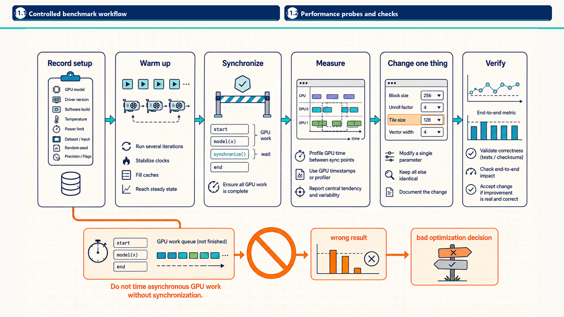
The main path records the environment and workload, warms up compilation and allocation, synchronizes the timed region, changes one factor, and checks both correctness and the measured metric. The warning path shows why unsynchronized timing can produce a false speedup and a bad engineering decision.

This chapter applies no new lever. It measures the ones already introduced, so that a claimed improvement can be separated from run-to-run variation. Section 1.6.1 lists the levers, and Section 1.6.2 gives the measurement workflow.

11.1 Controlled benchmark workflow

A valid comparison holds the workload, tensor shapes, software versions, and timing boundary constant. Framework warmup occurs separately so compilation and allocation do not enter the steady-state measurement.

11.1.1 Lab workflow and benchmark hygiene

A lab pass is one complete measurement cycle: define a bottleneck hypothesis, run controlled code, check correctness, collect evidence, and write an engineering conclusion. Benchmark hygiene is the discipline that keeps this cycle from measuring startup cost, shape drift, stale caches, or incorrect output instead of the intended performance question.

Procedure: Lab pass

A lab pass follows one fixed sequence:

1. Bottleneck hypothesis: The record states the suspected limiting resource.
2. Environment and workload: The record includes hardware, software, launch settings, and workload shapes.
3. Warmup boundary: Compilation, autotuning, allocation, and cache warmup finish outside the timed samples.
4. Shape policy: Shapes remain fixed unless shape variation is the factor under test.
5. Correctness evidence: Outputs, cache updates, gradients, or rank participation remain valid.
6. Timing method: Completed work is measured with the method that matches the question.
7. Interpretation: Evidence identifies one bottleneck class before a single factor changes.

11.1.2 Environment and version logging

An environment log is the reproducibility record for a performance result. It identifies the hardware, driver, runtime, framework, kernel backend, serving engine, and distributed launch context that produced the measurement.

• Hardware identity: GPU model, GPU count, memory capacity, interconnect, CPU model, and node shape.
• Driver/runtime identity: NVIDIA driver, CUDA runtime visible to PyTorch, cuDNN or attention backend versions when relevant.
• Framework identity: Python, PyTorch, Triton kernel-language/compiler, Transformers, serving engine, and distributed framework versions.
• Execution mode: Whether the run used eager execution, torch.compile, CUDA Graphs, quantization, custom kernels, or a serving-engine backend.

The experiment record includes Python, PyTorch, CUDA runtime, NVIDIA driver, GPU model, Triton kernel-language/compiler version, attention backend, serving engine version, and distributed launch configuration. Kernel availability, compiler behavior, quantized paths, and NCCL topology choices all depend on these versions. The following starter logger records common fields and makes missing optional packages explicit. The experiment-specific record also includes model, driver, topology, container, and benchmark settings.

Code example: Environment and version logger

import importlib.metadata
import os
import platform
import subprocess
import sys
import torch

def package_version(name):
    try:
        return importlib.metadata.version(name)
    except importlib.metadata.PackageNotFoundError:
        return "not installed"

print(f"Python: {sys.version.split()[0]}")
print(f"OS: {platform.platform()}")
print(f"PyTorch: {torch.__version__}")
print(f"CUDA runtime reported by PyTorch: {torch.version.cuda}")
print(f"cuDNN: {torch.backends.cudnn.version()}")
print(f"CUDA available: {torch.cuda.is_available()}")
if torch.cuda.is_available():
    props = torch.cuda.get_device_properties(0)
    print(f"GPU: {props.name}; memory={props.total_memory / 2**30:.1f} GiB")

for package in ("triton", "transformers", "flash-attn", "xformers", "vllm", "deepspeed"):
    print(f"{package}: {package_version(package)}")

for name in ("CUDA_VISIBLE_DEVICES", "RANK", "LOCAL_RANK", "WORLD_SIZE", "NCCL_SOCKET_IFNAME"):
    print(f"{name}={os.environ.get(name, '<unset>')}")

try:
    driver = subprocess.run(
        ["nvidia-smi", "--query-gpu=driver_version", "--format=csv,noheader"],
        check=True, capture_output=True, text=True,
    ).stdout.splitlines()[0]
except (FileNotFoundError, subprocess.CalledProcessError, IndexError):
    driver = "unavailable"
print(f"NVIDIA driver: {driver}")

The logger distinguishes the CUDA runtime bundled or reported by PyTorch from the installed NVIDIA driver. Package versions establish which compiler, attention, serving, and distributed paths were available. Environment variables record device visibility and rank placement. A final experiment record should also include model revision, input-shape distribution, precision, compiler mode, cache settings, launch command, and the profiler or timing method.

11.1.3 Warmup policy and shape control

Warmup is the deliberate execution of unmeasured iterations before timing begins. It initializes kernels, allocator state, autotuning, graph compilation, and serving-engine caches so the measurement reflects steady-state behavior rather than first-run setup.

Shape control means deciding which tensor dimensions are allowed during a benchmark: batch size, sequence length, hidden size, head dimension, and the mix of prefill and decode tokens. It matters because torch.compile, CUDA Graphs, attention kernels, and serving schedulers often specialize to dimension ranges. If production sequence lengths vary, benchmark their actual distribution.

• Warmup count: Enough unmeasured iterations to trigger compilation, autotuning, allocator growth, and cache creation.
• Static-shape experiment: Keeps shapes fixed to isolate kernel, compiler, or CUDA Graph behavior.
• Variable-shape experiment: Uses a controlled distribution of lengths or batch shapes to test scheduler and compiler behavior under realistic variability.
• Shape drift: An accidental change in tensor dimensions between runs, often causing recompilation or different kernel selection.

Warmup removes one-time setup from steady-state timing, while deliberate shape control determines whether recompilation and kernel changes belong to the experiment. The next question is whether the candidate path still computes the intended result across that chosen shape range.

11.1.4 Correctness checks

A correctness check verifies that the optimized path still computes the intended result. Performance numbers are not useful if a kernel silently drops work, a decode loop corrupts the cache, or a distributed job leaves some ranks out of the computation.

• Custom kernel: A PyTorch reference supplies expected outputs. The experiment chooses a tolerance appropriate to the dtype, operation, and error budget.
• Decode path: Generated shapes, appended tokens, and key-value cache updates remain valid.
• Distributed job: All ranks participate, gradients update, and cleanup runs even after an exception.

torch.allclose provides a simple floating-point comparison when an optimized tensor output should match an eager reference. This abbreviated snippet expects optimized_output and eager_reference to be same-shaped tensors. Its input is that tensor pair, and its result is assertion success or failure. For each output value \(a\) and reference value \(b\), the condition is \(|a-b|\leq10^{-3}+10^{-3}|b|\). NaNs fail this default comparison¹:

Code example: Floating-point correctness check

import torch

# Verify optimized output matches eager reference within tolerance
assert torch.allclose(optimized_output, eager_reference, rtol=1e-3, atol=1e-3), \
    f"Mismatch! Max absolute difference: {(optimized_output - eager_reference).abs().max()}"

Tolerance is part of the correctness contract. A fused or lower-precision path may differ bit-for-bit from a reference path, so the allowed error must be chosen before timing and before any surprising speedup appears.

For serving experiments, correctness also includes sequence-level behavior: the cache should grow as expected, finished requests should stop advancing, and batching should not change the requested decoding constraints.

11.1.5 Benchmark harness structure

A benchmark harness is the wrapper code that prepares inputs, runs warmup, measures the intended region, checks correctness, and reports results. Its job is to make the measurement reproducible and to keep setup or teardown work out of the timing window.

A small harness should separate responsibilities instead of hiding them inside one timing block:

• Setup: Inputs, the model or engine, and the device are constructed before the measured region.
• Warmup: Unmeasured iterations initialize kernels, compilation paths, caches, and allocator state.
• Measurement: The timed region answers the bottleneck question and excludes setup.
• Synchronization: torch.cuda.synchronize() brackets measured CUDA work when wall-clock timing is required.
• Reporting: Serving experiments report both latency and throughput because a scheduler can improve one while harming the other.

CUDA events measure elapsed time between two points on a CUDA stream. They omit host work outside that interval, but include idle gaps inside it if the host fails to enqueue the next operation in time. They are appropriate for device-stream timing rather than end-to-end latency². This abbreviated snippet expects model, inputs, warmup_steps, and a positive num_steps to be bound. Its input is the model and data, and its output is printed elapsed time in milliseconds. A valid result requires synchronization before measurement and after the loop:

Code example: CUDA event timing loop

import torch

# 1. Warmup
for _ in range(warmup_steps):
    _ = model(inputs)
torch.cuda.synchronize()

# 2. Synchronized timing loop
start_event = torch.cuda.Event(enable_timing=True)
end_event = torch.cuda.Event(enable_timing=True)

start_event.record()
for _ in range(num_steps):
    _ = model(inputs)
end_event.record()

torch.cuda.synchronize()
elapsed_ms = start_event.elapsed_time(end_event)
print(f"Average step latency: {elapsed_ms / num_steps:.2f} ms")

The event result measures elapsed time between recorded stream events, including any intervening stalls. End-to-end latency also includes a synchronized wall-clock measurement of host dispatch, scheduling, copies, and waits outside the stream interval. A serving harness additionally fixes arrivals, outstanding-request limits, cache state, and outcome accounting using the request-load experiment in Section 10.8. GPU-loop timing alone cannot measure request queueing or service goodput.

11.1.6 Profiler selection guide

Profiler selection is a layer-selection decision: the tool collects evidence at the layer where the hypothesis lives. Section 5.4.1 compares PyTorch Profiler, Nsight Systems, Nsight Compute, and Perfetto by the question each answers.

A trace reveals CPU-side tokenization, API work, GPU idle gaps, many tiny kernels, memory copies, synchronization points, and the separation between long prefill regions and repeated decode steps.

11.1.7 Interpretation template

Reading results means connecting the measurement to a bottleneck class. A useful result note contains five parts:

• Measured result: What the profiler, benchmark, or trace actually showed.
• Likely bound: Memory-bound, compute-bound, launch-bound, communication-bound, or scheduler-bound.
• Supporting evidence: The counter, trace region, timeline gap, or formula that supports the suspected cause.
• Next change: The smallest change that should move the identified bottleneck.
• Other cause checked: The other plausible cause considered and the evidence that points elsewhere.

This keeps profiler tables from becoming isolated numbers. A good result note states what happened, what should change next, and what evidence would disprove that next step.

The template is completed immediately after the run while the trace, command line, and environment log are still available. Otherwise the result becomes difficult to compare with the next experiment.

11.1.8 Reliable measurement

Reliable GPU measurement matches the timing method to the question being asked. The following checklist keeps Python timing, asynchronous CUDA execution, first-run compilation, shape variation, and scheduler effects from changing the measured quantity.

Checklist: Reliable measurement

• Wall-clock GPU timing is synchronized when the metric is device execution time.
• First-run compilation or autotuning is reported separately from steady-state latency.
• Tensor shapes remain fixed when one change is compared, or shape variation is reported as an independent factor.
• Expected workload sizes expose the target memory pressure or communication overhead.
• The serving-latency distribution, including tail latency, is reported when the service target depends on it.
• Multiple repeated samples provide statistics rather than a single trial.
• Timeline and stream dependencies establish copy, communication, and compute overlap.
• GPU clocks, power limits, and throttling events are recorded, and clocks are locked for microbenchmarks where the system permits it.

GPU clocks are a hidden variable. A GPU raises and lowers its clock with temperature and power draw, so two runs of the same kernel can differ because one was throttled. nvidia-smi can lock the GPU clock to a fixed range (--lock-gpu-clocks) and set a power limit (--power-limit), both of which need administrator rights, and its clock-event reasons report when the software power cap or a thermal slowdown reduced the clock.³ A microbenchmark that compares two kernels runs at locked clocks where permitted. An end-to-end benchmark records the clocks and throttle reasons it saw, because production runs at whatever clock the hardware chooses.

Synchronization makes wall-clock GPU timing cover completed device work. Separate warmup and controlled shapes keep repeated measurements comparable. For a service endpoint, the Section 10.8 load contract also fixes request times independently of replies and includes rejected and unfinished requests in the report. Both configurations must use the same arrival policy and observation window.

11.1.9 Runtime setup and launch configuration

Runtime setup is the set of process-level choices that change how the benchmark executes. Distributed launch settings (ranks, torchrun, and NCCL variables) are covered in Section 12.8.1. The environment log records what system produced a result. Runtime setup controls which devices are visible, how memory allocation behaves, which distributed launcher creates ranks, and which diagnostics are enabled.

These controls are set before timing begins. A benchmark launched with different visible GPUs, allocator policy, NCCL interface, or distributed rank mapping is a different experiment even if the Python model code is identical.

• CUDA_VISIBLE_DEVICES controls which GPUs the process can see and how they are enumerated.
• PYTORCH_CUDA_ALLOC_CONF changes caching allocator behavior and is useful when fragmentation is suspected.

Runtime variables and launch tools define the visible devices, allocator, rank mapping, and transport path, so changing them creates a different experiment even when model code is unchanged. The next question is how to apply the same controlled sequence to recurring roofline, decode, compilation, and communication tests.

11.1.10 Recurring experiment patterns

Several experiment shapes recur across performance work. They differ in the measured object, but they share the same discipline: establish a baseline, change one mechanism, verify the output, and explain the result using evidence from the appropriate software and hardware layer.

• Roofline exercise pattern: The exercise counts FLOPs, estimates HBM bytes, measures steady-state time, computes arithmetic intensity, compares bandwidth and compute ceilings, and explains any contradiction.
• Decode optimization pattern: The pattern separates prefill from repeated decode, validates KV-cache updates, measures per-token latency, and tests whether the next bottleneck is memory bandwidth, launch overhead, or scheduler gaps.
• Compile and CUDA Graph pattern: The pattern warms up, identifies graph breaks, stabilizes shapes and memory addresses, captures only steady GPU work, replays it, and compares it with eager execution without including compile time.
• Speculative-decoding pattern: The evidence set includes draft tokens, target verification, retained-prefix lengths, committed token counts, gamma, and measured wall time together. Theoretical alpha and c belong to the separate cost-model estimate. Acceptance is not interpretable without wall-clock evidence.
• Interpretation discipline: Working code becomes evidence only after its assumptions, timing boundary, and correctness check are explicit. The point is to explain why each measurement step exists.

A good lab write-up therefore ends with an engineering conclusion: which resource bounded the run, what evidence supports that conclusion, what change should move the bound, and which tempting change is unlikely to help.

11.2 Performance probes and checks

Each template below is a controlled probe for one bottleneck question. The mechanism it exercises is taught in the section linked beside it. The notes here add the input shapes the template assumes, its correctness check, and what its output shows.

11.2.1 PyTorch profiling template

The first PyTorch profiling pass establishes the hot operations before a change is made. PyTorch’s native profiler uses a context manager to trace host CPU thread execution, CUDA API dispatch, and GPU kernel execution timelines.

Worked example: PyTorch profiling template

This profile records several steady-state iterations after an explicit wait and warmup schedule. The aggregate table identifies expensive framework operations. The trace supplies the timing relationships needed to distinguish kernel time from launch gaps, copies, and synchronization.

Code example: PyTorch profiling template

import torch
from torch.profiler import ProfilerActivity, profile, schedule

device = torch.device("cuda", 0)
args = (torch.randn(1024, 1024, device=device),)
def fn(x):
    return torch.relu(x @ x)

for _ in range(5):
    fn(*args)

with profile(
    activities=[ProfilerActivity.CPU, ProfilerActivity.CUDA],
    schedule=schedule(wait=1, warmup=1, active=3, repeat=1),
    record_shapes=True,
    profile_memory=True,
    on_trace_ready=torch.profiler.tensorboard_trace_handler("./traces"),
) as prof:
    for _ in range(5):
        fn(*args)
        prof.step()
print(prof.key_averages().table(sort_by="cuda_time_total", row_limit=20))

The table ranks framework operations within the selected profiling window. A large CUDA total points to where device time accumulates, while the timeline shows whether that time comes from long kernels, repeated short launches, copies, synchronization, or idle gaps. Memory coalescing cannot be diagnosed from a CPU-to-GPU gap. It requires kernel-level memory-transaction evidence.

For ordering across CPU and GPU lanes, the system timeline tools of Section 5.4.1 take over.

11.2.2 Timeline tracing

Operator totals identify expensive framework calls, but they do not show whether delay occurs in host scheduling, CUDA submission, memory copies, device kernels, or communication. A system timeline preserves that ordering. The two workflows below capture it through Nsight Systems or export it for Perfetto.

Worked example: Nsight Systems capture

This command records a system-level timeline around the real training or serving entry point. The output report correlates operating-system scheduling, CUDA API calls, library calls, kernels, memory copies, and NVTX ranges.

Code example: Nsight Systems capture

nsys profile --trace=cuda,nvtx,osrt,cublas,cudnn \
  --sample=none \
  -o run_trace python train_or_serve.py

Worked example: PyTorch trace export for Perfetto

This second path exports a Chrome-trace JSON from a complete PyTorch Profiler schedule. Perfetto can then inspect the CPU and CUDA lanes in a browser without changing the measurement boundary used by the profiler.

Code example: PyTorch trace export for Perfetto

import torch
from torch.profiler import ProfilerActivity, profile, schedule

with profile(
    activities=[ProfilerActivity.CPU, ProfilerActivity.CUDA],
    schedule=schedule(wait=1, warmup=1, active=3, repeat=1),
    on_trace_ready=lambda p: p.export_chrome_trace("trace.json"),
) as prof:
    for _ in range(5):
        train_or_serve_step()
        prof.step()
# Open trace.json in https://ui.perfetto.dev.

Empty GPU intervals show that no GPU work was executing, but the timeline must identify why. Possible causes include CPU dispatch, compilation, input starvation, a synchronization dependency, communication, memory allocation, or intentional waiting. The surrounding CPU, CUDA API, copy, and collective lanes provide the distinguishing evidence.

Arithmetic intensity places the measured kernel under either the bandwidth ceiling or the compute ceiling. That placement identifies the first bottleneck hypothesis. Achieved bandwidth, occupancy, launch timing, and memory-transaction counters are still needed before choosing an optimization.

11.2.3 Roofline calculation template

Worked example: 11.2.3 Roofline calculation template

This Python example turns a measured kernel into a roofline point. It includes sample numbers so the output can be interpreted immediately. Supply nonnegative FLOP and byte counts, positive elapsed time and hardware rates, and a positive HBM byte count for a finite arithmetic intensity. The arithmetic helper does not validate these input domains.

Code example: Roofline calculation template

def roofline(flops, bytes_moved, seconds, peak_tflops, peak_tb_s):
    ai = flops / bytes_moved
    achieved = flops / seconds / 1e12
    memory_ceiling = ai * peak_tb_s
    bound = min(peak_tflops, memory_ceiling)
    bound_type = "memory-bound" if memory_ceiling < peak_tflops else "compute-bound"
    return ai, achieved, bound, bound_type

ai, achieved, bound, bound_type = roofline(
    flops=2e12,
    bytes_moved=1e12,
    seconds=0.500,
    peak_tflops=200,
    peak_tb_s=3,
)
print(f"AI={ai:.1f} FLOPs/byte, achieved={achieved:.1f} TFLOP/s")
print(f"roofline_bound={bound:.1f} TFLOP/s, bound_type={bound_type}")

With the sample inputs, arithmetic intensity is 2 FLOPs per byte, the HBM ceiling is 6 TFLOP/s, and achieved throughput is 4 TFLOP/s. The point is below the memory roof and cannot yet be called bandwidth-saturated. A trace and kernel counters are needed to determine whether launch overhead, occupancy, access efficiency, or another dependency explains the remaining gap.

The next template reruns the Triton GEMV kernel of Section 4.5 across tile sizes.

It applies when profiler evidence shows a layout or fusion opportunity beyond the selected vendor or compiler path.

11.2.4 Triton GEMV kernel

Worked example: 11.2.4 Triton GEMV kernel

This Triton matrix-vector multiplication probe requires a CUDA-enabled PyTorch installation, a supported NVIDIA GPU, and an installed Triton version compatible with that PyTorch release. It shows program IDs, tile offsets, masked loads, reductions, and stores. Inputs are converted to FP32 before multiplying and accumulating. A wider FP64 PyTorch calculation supplies the reference, then the result is compared in the output’s FP32 dtype. Each candidate BLOCK value is launched and checked against that same reference before its own timing begins. A failed comparison prints the candidate and skips its timing. The example tolerances allow reduction-order differences for these inputs. A different value range may need a separate error analysis. The fixed inputs and tolerances apply to all three candidates, so only configurations that pass the check enter the timing comparison.

Code example: Triton GEMV kernel

import torch
import triton
import triton.language as tl

if not torch.cuda.is_available():
    raise RuntimeError("This benchmark requires CUDA-enabled PyTorch")

@triton.jit
def gemv_kernel(A, x, y, M: tl.constexpr, N: tl.constexpr, BLOCK: tl.constexpr):
    row = tl.program_id(0)
    offsets = tl.arange(0, BLOCK)
    acc = tl.full((), 0.0, tl.float32)
    for start in range(0, N, BLOCK):
        cols = start + offsets
        mask = cols < N
        acc += tl.sum(tl.load(A + row * N + cols, mask=mask, other=0.0).to(tl.float32)
                      * tl.load(x + cols, mask=mask, other=0.0).to(tl.float32), axis=0)
    tl.store(y + row, acc)
M, N = 4096, 4096
A = torch.randn((M, N), device="cuda", dtype=torch.float16)
x = torch.randn((N,), device="cuda", dtype=torch.float16)
y = torch.empty((M,), device="cuda", dtype=torch.float32)
reference = (A.double() @ x.double()).float()
for block in (256, 512, 1024):
    gemv_kernel[(M,)](A, x, y, M, N, BLOCK=block)
    try:
        torch.testing.assert_close(y, reference, rtol=1e-4, atol=1e-3)
    except AssertionError as error:
        print(f"BLOCK={block}: correctness failed; timing skipped: {error}")
        continue
    ms = triton.testing.do_bench(
        lambda block=block: gemv_kernel[(M,)](A, x, y, M, N, BLOCK=block)
    )
    print(f"BLOCK={block}: {ms:.3f} ms")

Definition - Code-to-object mapping

A: The matrix with shape M by N. In a decode-like projection, this stands for a large weight matrix read from GPU memory.

x: The vector with length N. This stands for one token representation or a small batch slice.

row: The Triton program id. One program computes one output coordinate y[row].

offsets and mask: The tile-local column indices and boundary guard. They define which elements of A[row, :] and x are read in each loop chunk.

acc: The running dot-product accumulator for y[row], kept in registers or fast local storage before the final store.

This kernel is a controlled row-wise baseline, not a claim that custom Triton always beats the selected library or compiler path. Nsight Compute exposes memory transactions, achieved bandwidth, occupancy, and register pressure for the fastest correct configuration. That configuration is compared with the production operator on the same shape and dtype.

The attention comparison that follows measures the memory saving explained in Section 4.8.

11.2.5 Attention backend comparison

Worked example: 11.2.5 Attention backend comparison

The naive path materializes B x H x S x S score and probability tensors. The optimized call requests the FlashAttention backend. The check below compares outputs, event time, and additional allocated memory for one forward-only shape. This comparison applies only on a CUDA configuration that supports the requested backend. The forced-backend call catches and records an error if this configuration cannot use FlashAttention, then skips the comparison. It does not silently fall back to another attention backend.

Code example: Attention backend comparison

import gc
import torch
import torch.nn.functional as F
from torch.nn.attention import SDPBackend, sdpa_kernel

# Shapes: Batch, Heads, Sequence Length, Head Dimension
B, H, S, D = 4, 32, 2048, 128
q = torch.randn(B, H, S, D, device="cuda", dtype=torch.float16)
k = torch.randn(B, H, S, D, device="cuda", dtype=torch.float16)
v = torch.randn(B, H, S, D, device="cuda", dtype=torch.float16)

# 1. Naive Attention (explicit O(S squared) intermediate matrix)
def naive_attention(q, k, v):
    scale = 1.0 / (q.shape[-1] ** 0.5)
    attn_weights = torch.matmul(q, k.transpose(-2, -1)) * scale
    attn_probs = F.softmax(attn_weights, dim=-1)
    return torch.matmul(attn_probs, v)

# 2. Optimized scaled-dot-product attention backend
def optimized_attention(q, k, v):
    with sdpa_kernel(SDPBackend.FLASH_ATTENTION):
        return F.scaled_dot_product_attention(q, k, v)

@torch.inference_mode()
def measure(fn, repeats=10):
    gc.collect()
    torch.cuda.empty_cache()
    for _ in range(3):
        out = fn(q, k, v)
    torch.cuda.synchronize()
    baseline = torch.cuda.memory_allocated()
    torch.cuda.reset_peak_memory_stats()
    start = torch.cuda.Event(enable_timing=True)
    stop = torch.cuda.Event(enable_timing=True)
    start.record()
    for _ in range(repeats):
        out = fn(q, k, v)
    stop.record()
    torch.cuda.synchronize()
    extra_peak = torch.cuda.max_memory_allocated() - baseline
    return out, start.elapsed_time(stop) / repeats, extra_peak

naive_out, naive_ms, naive_peak = measure(naive_attention)
try:
    flash_out, flash_ms, flash_peak = measure(optimized_attention)
except RuntimeError as error:
    print(f"flash: unsupported; comparison skipped: {error}")
else:
    torch.testing.assert_close(flash_out, naive_out, rtol=2e-2, atol=2e-2)
    print(f"naive: {naive_ms:.3f} ms, extra peak {naive_peak / 2**20:.1f} MiB")
    print(f"flash: {flash_ms:.3f} ms, extra peak {flash_peak / 2**20:.1f} MiB")

Definition - Code-to-object mapping

q, k, v: Query, key, and value tensors with shape B by H by S by D.

attn_weights: The explicit B by H by S by S score tensor in the naive implementation. This is the object FlashAttention avoids materializing in HBM.

attn_probs: The normalized score tensor after softmax. In the naive path it is another large intermediate. In the tiled path its effect is computed online.

F.scaled_dot_product_attention: The PyTorch API call that may dispatch to a FlashAttention-style backend when dtype, device, mask, and shape constraints are compatible.

The explicit score matrix alone contains B times H times S squared elements, but the measured peak also depends on allocator reuse, outputs, temporary workspaces, and backend implementation. Evidence across representative sequence lengths includes unsupported shapes or fallbacks. One successful configuration does not establish behavior for every attention workload.

The next probe tests the graph-break behavior described in Section 6.3 on the installed PyTorch version.⁴

The small branch isolates one boundary. In larger serving or training code, the same boundary appears as logging, shape-dependent Python decisions, sampling logic placed inside the model step, or scalar diagnostics mixed into the hot tensor path.

11.2.6 Inspecting a torch.compile boundary

Worked example: 11.2.6 Inspecting a torch.compile boundary

This example contrasts a tensor-valued selection with a Python branch driven by a CUDA scalar. Both functions are compiled and executed so graph-break diagnostics can report the behavior of the installed PyTorch configuration.

Code example: Inspecting a torch.compile boundary

import torch

# Normal compiled path: condition remains a GPU tensor
def compiled_step(x):
    return torch.where(x.sum() > 0, x * 2, x - 2)

compiled = torch.compile(compiled_step, mode="reduce-overhead")
x = torch.randn(1024, device="cuda")
y = compiled(x)

# Host-control variation: .item() returns a Python scalar.
def host_branch(x):
    return x * 2 if x.sum().item() > 0 else x - 2

compiled_host_branch = torch.compile(host_branch)
z = compiled_host_branch(x)

The diagnostic run uses TORCH_LOGS='graph_breaks,recompiles' or the current PyTorch diagnostic interface. Its record contains observed captured regions, fallbacks, recompilations, and steady-state time for the installed version and input shapes, rather than an assumed break count.

The CUDA Graph template applies the capture and replay rules of Section 6.5 to a module.

11.2.7 CUDA Graph warmup and replay

Worked example: 11.2.7 CUDA Graph warmup and replay

This inference-mode pattern warms the module on a side stream, synchronizes before capture, records stable-address work, and explains the lifetime of the captured output buffer. It applies after profiling shows launch overhead and the shapes and addresses can remain stable.

Code example: CUDA Graph warmup and replay

import torch

device = torch.device("cuda", 0)
module = torch.nn.Linear(1024, 1024).to(device).eval()
example = torch.randn(32, 1024, device=device)
graph = torch.cuda.CUDAGraph()
static_in = torch.empty_like(example)
warmup_stream = torch.cuda.Stream()

with torch.inference_mode():
    warmup_stream.wait_stream(torch.cuda.current_stream())
    with torch.cuda.stream(warmup_stream):
        for _ in range(3):
            _ = module(static_in)
    torch.cuda.current_stream().wait_stream(warmup_stream)
    torch.cuda.synchronize()

    with torch.cuda.graph(graph):
        static_out = module(static_in)

@torch.inference_mode()
def replay(x, *, keep_snapshot=False):
    if x.shape != static_in.shape or x.dtype != static_in.dtype or x.device != static_in.device:
        raise ValueError("x must match static_in shape, dtype, and device exactly")
    static_in.copy_(x)
    graph.replay()
    return static_out.clone() if keep_snapshot else static_out

Capture safety is workload-specific: lazy initialization, unsupported operations, dynamic allocations, changing shapes, or cross-stream dependencies can make a sequence unsafe. Each replacement input must have the captured input’s shape, dtype, and device. The template checks those properties before copy_ because copy_ itself can broadcast or convert other inputs⁵. Replay is compared with a warmed eager or compiled baseline, and compilation time remains separate from steady-state replay time.

The cached-decode probe traces the state flow explained in Section 9.1 and returns the generated tokens so its behavior can be checked.

11.2.8 Cached decode state

Worked example: 11.2.8 Cached decode state

This callable PyTorch probe takes nonempty token IDs shaped [B, P], an integer generation limit, and optionally one EOS token ID. It assumes unpadded equal-length prompts and a compatible Hugging Face Transformers model in evaluation mode that accepts past_key_values and infers positions from the cache, as in Section 9.1. Models requiring explicit masks or cache-position arguments need an adapted wrapper.

EOS stopping is supported only for batch size one. Supplying an EOS ID with B > 1 raises ValueError before any model call. With no EOS ID, the probe generates a fixed number of tokens for every row and does not stop at EOS. A nonpositive limit returns shape [B, 0]. The output contains only new token IDs, including EOS when it triggers stopping. The first call processes the prompt and creates the cache. Later calls consume the previous selected token plus that cache, then predict the next token.

For example, let one prompt contain three tokens and the greedy choices be token 7 followed by EOS, with a limit of four. Prefill caches the three prompt positions and selects 7. One further call consumes 7, extends the cache to four positions, and selects EOS. The function returns [7, EOS] and makes no further model call. The final selected token has not been fed back into the model, and the function returns no cache. This is a state-flow probe, not a complete serving scheduler or sampler.

Code example: Cached decode state

import torch
@torch.inference_mode()
def cached_decode(model, input_ids, max_new_tokens, eos_token_id=None):
    if input_ids.ndim != 2 or input_ids.shape[0] == 0 or input_ids.shape[1] == 0:
        raise ValueError("input_ids must have nonempty shape [B, P]")
    if eos_token_id is not None and input_ids.shape[0] != 1:
        raise ValueError("EOS stopping requires batch size one")
    if max_new_tokens <= 0:
        return input_ids[:, :0]
    out = model(input_ids, use_cache=True)
    past = out.past_key_values
    token = out.logits[:, -1].argmax(dim=-1, keepdim=True)
    generated = [token]
    for _ in range(max_new_tokens - 1):
        if eos_token_id is not None and token.item() == eos_token_id:
            break
        out = model(token, past_key_values=past, use_cache=True)
        past = out.past_key_values
        token = out.logits[:, -1].argmax(dim=-1, keepdim=True)
        generated.append(token)
    return torch.cat(generated, dim=1)

Definition - State trace

Prefill call: model(input_ids, use_cache=True) processes the prompt and returns the initial cache for all layers.

past: The persistent decode state. Its token dimension grows as generation proceeds, so cache reads still scale with context length.

token: A one-token tensor fed to later model calls. The compute for new Q/K/V is small, but attention reads the stored K/V history.

Updated cache: Each post-prefill model call adds the previous selected token’s keys and values. Selection alone does not add that newly predicted token to the cache. The EOS check can stop before another cache update.

Preserving key-value states shifts the decode workload from recomputing the whole prefix toward reading and extending stored attention state. In this case, optimization must focus on cache capacity, layout, transfer bandwidth, and launch overhead rather than treating decode as constant-cost arithmetic.

The calculator implements the KV-cache formula of Section 8.6. It estimates packed scalar storage only, before block metadata, scale tensors, padding, fragmentation, allocator reserves, and temporary workspaces.

11.2.9 Key-value cache lower-bound calculator

Worked example: 11.2.9 Key-value cache lower-bound calculator

This Python calculator estimates raw packed KV storage from batch size, stored sequence length, layer count, key-value heads, head dimension, and bits per element. Supply nonnegative integer batch size and sequence length, positive integer layer and head counts and head dimension, and a positive bit width. The helper does not validate those domains. It reports binary GiB and deliberately keeps storage-format overhead outside the formula.

Code example: Key-value cache lower-bound calculator

def estimate_kv_cache_gib(batch_size, seq_len, layers, kv_heads, head_dim, bits_per_element=16):
    # 2 for separate Key and Value states
    elements_per_token = layers * kv_heads * head_dim * 2
    total_elements = batch_size * seq_len * elements_per_token
    total_bytes = total_elements * bits_per_element / 8
    return total_bytes / (1024 ** 3)

gib = estimate_kv_cache_gib(
    batch_size=32,
    seq_len=4096,
    layers=32,
    kv_heads=8,      # Grouped-Query Attention (GQA)
    head_dim=128,
    bits_per_element=16,  # FP16/BF16 scalar payload
)
print(f"Raw packed KV payload: {gib:.2f} GiB")

Definition - Code-to-formula mapping

batch_size: B, the number of active sequences admitted by the scheduler.

seq_len: S, the number of stored prompt plus generated tokens per sequence.

layers: L, the number of transformer layers that keep KV state.

kv_heads and head_dim: The key-value head count and per-head dimension in the KV-cache formula.

bits_per_element: The nominal packed payload width of each cached scalar. It is not a complete quantized-storage model.

gib: The raw KV-cache payload converted to GiB. It excludes block metadata, scales, padding, fragmentation, and temporary workspaces.

The next reference implementation follows the acceptance and correction rules of Section 10.6 for one sequence, without KV-cache reuse.

11.2.10 Distribution-correct speculative step

Worked example: 11.2.10 Distribution-correct speculative step

This pedagogical implementation drafts k tokens, verifies them in one target-model pass, applies the standard acceptance rule, and commits either a residual-sampled correction or one additional target token. It deliberately recomputes model state and uses host-visible decisions, so it is a correctness reference rather than a production speed implementation. The template needs real compatible checkpoint IDs in place of its two placeholders, a nonempty tokenized prompt, and a positive integer k. It uses plain categorical sampling with FP32 probability calculations. Finite precision can still differ from the exact-arithmetic distribution proof.

Code example: Distribution-correct speculative step

import time
import torch
from transformers import AutoTokenizer, AutoModelForCausalLM

device = torch.device("cuda", 0)
target_name = "target-checkpoint"
draft_name = "draft-checkpoint"

tokenizer = AutoTokenizer.from_pretrained(target_name)
draft_tokenizer = AutoTokenizer.from_pretrained(draft_name)
target = AutoModelForCausalLM.from_pretrained(
    target_name, torch_dtype=torch.float16
).to(device).eval()
draft = AutoModelForCausalLM.from_pretrained(
    draft_name, torch_dtype=torch.float16
).to(device).eval()
if (
    tokenizer.get_vocab() != draft_tokenizer.get_vocab()
    or tokenizer.special_tokens_map != draft_tokenizer.special_tokens_map
):
    raise ValueError("Draft and target require the same token-to-ID mapping")

@torch.inference_mode()
def speculative_step(prompt, k=4):
    if isinstance(k, bool) or not isinstance(k, int) or k < 1:
        raise ValueError("k must be a positive integer")
    input_ids = tokenizer(prompt, return_tensors="pt").input_ids.to(device)
    prompt_len = input_ids.shape[1]
    if prompt_len == 0:
        raise ValueError("prompt must contain at least one token")
    draft_ids = input_ids
    draft_probs = []

    torch.cuda.synchronize()
    start = time.perf_counter()
    for _ in range(k):
        q_logits = draft(draft_ids, use_cache=False).logits[:, -1]
        q_probs = torch.softmax(q_logits.float(), dim=-1)
        next_id = torch.multinomial(q_probs, num_samples=1)
        draft_probs.append(q_probs)
        draft_ids = torch.cat([draft_ids, next_id], dim=1)

    target_logits = target(draft_ids, use_cache=False).logits
    accepted = 0
    committed = None
    for i, pos in enumerate(range(prompt_len, draft_ids.shape[1])):
        token = draft_ids[:, pos]
        p = torch.softmax(target_logits[:, pos - 1].float(), dim=-1)
        q = draft_probs[i]
        ratio = p.gather(1, token[:, None]) / q.gather(1, token[:, None])
        accept = (torch.rand_like(ratio) < torch.clamp(ratio, max=1.0)).item()
        if accept:
            accepted += 1
        else:
            residual = torch.clamp(p - q, min=0)
            residual_mass = residual.sum(dim=-1, keepdim=True)
            if not torch.isfinite(residual_mass).all() or (residual_mass <= 0).any():
                raise RuntimeError("Nonpositive or nonfinite residual mass after rejection")
            residual = residual / residual_mass
            replacement = torch.multinomial(residual, num_samples=1)
            committed = torch.cat([draft_ids[:, :pos], replacement], dim=1)
            break

    if committed is None:
        extra_p = torch.softmax(target_logits[:, -1].float(), dim=-1)
        extra_token = torch.multinomial(extra_p, num_samples=1)
        committed = torch.cat([draft_ids, extra_token], dim=1)

    torch.cuda.synchronize()
    wall_ms = (time.perf_counter() - start) * 1000
    return committed, accepted, wall_ms

Definition - Code-to-object mapping

draft_ids: The growing candidate sequence proposed by the draft model.

draft_probs: The saved draft distributions q(x) at the exact positions where candidate tokens were proposed.

target_logits and p: The target-model verification output and target distribution p(x).

ratio: The p(x) / q(x) term used by the acceptance rule for the proposed token.

accepted: The retained draft-prefix length, an integer from 0 through k. Its average is the mean accepted-prefix length, not the theoretical probability alpha. Dividing that mean by k does not establish alpha either, because proposals after the first rejection are not retained.

committed: The prompt plus the accepted prefix and either a residual correction or an extra target-sampled token.

wall_ms: Synchronized wall time for this unoptimized reference step. Compare it with a target-only reference on the same prompts before claiming speedup.

Worked example: Reporting speculative progress

Consider three illustrative calls with k = 4 and returned accepted-prefix lengths 0, 2, and 4. Their mean is (0 + 2 + 4) / 3 = 2 draft tokens per call. Each call also commits a residual correction or an extra target token, so the corresponding new-token counts are 1, 3, and 5. These counts can be checked directly by subtracting the original prompt length from each returned sequence length.

Suppose the synchronized step times are 12, 15, and 18 ms. The combined result is nine new tokens in 45 ms, or 9 / 0.045 = 200 tokens/s across these measured step intervals. This is illustrative arithmetic, not an observed benchmark. The ratio of total tokens to total time weights the intervals correctly. An unweighted mean of per-call rates would answer a different question.

The timing excludes loading and tokenization but includes this reference’s draft work, target verification, sampling, and tensor updates. It is not endpoint goodput. The reference has no EOS or output-budget truncation. A serving implementation must count only tokens actually committed before stopping. Separate reports by k and prompt class make changes in workload visible. A matched target-only run must generate the same number of new tokens under the same output rules and timing boundary before a speedup ratio is meaningful.

The Chapter 10 cost model uses a theoretical alpha with independent acceptance assumptions. No estimator of that parameter is inferred from these stopped-prefix counts. This reference omits KV-cache reuse, rollback, batching, and device-side acceptance, so its elapsed time does not establish production speed.

The final template batches that verification across sequences, as production decoders do (Section 10.6).

11.2.11 Vectorized speculative verification

Worked example: 11.2.11 Vectorized speculative verification

This pseudocode fixes the data contract for batched verification. It assumes B nonempty, unpadded prompts of common length P, k >= 1 proposals, identical draft/target token IDs, and plain categorical sampling from normalized probabilities over vocabulary size V. It recomputes full prefixes without persistent caches to make position alignment explicit. No EOS stopping or output-budget truncation is applied here.

draft_ids contains the prompt plus proposals, shape [B, P+k]. proposal_ids is only the [B, k] suffix. draft_probs, shape [B, k, V], stores the full distribution used at each proposal position. The target output has shape [B, P+k, V]. Its logits at P-1+i predict proposal i, and its final logits predict an extra token after all k proposals. The gathered [B, k] proposal probabilities are sufficient for acceptance decisions, but residual sampling needs both full vocabulary distributions at the first rejection.

For a row retaining n < k proposals, the commit helper uses target_probs[row, n, :] and draft_probs[row, n, :], normalizes max(p - q, 0), and samples one correction. For n = k, it samples from extra_target_probs[row, :]. It returns that row’s original prompt, the n retained proposals, and this one final token as a variable-length sequence. A zero residual mass on an actual rejection is a numerical error to report, not permission to substitute ordinary target sampling. Production integration additionally needs per-request stopping, output limits, and cache rollback.

Code example: Vectorized speculative verification

# Pseudocode: B equal-length unpadded prompts, plain categorical sampling.
# propose returns full prompt + k tokens and the full q used for each draw.
B, P = input_ids.shape                         # P >= 1; k >= 1
draft_ids, draft_probs = draft_model.propose(input_ids, k=k)
proposal_ids = draft_ids[:, P:]                # [B, k]
# draft_ids: [B, P+k]; draft_probs: [B, k, V]
# Full-prefix computation here; no persistent KV state is passed or returned.
target_logits = target_model(draft_ids, use_cache=False).logits
target_probs = target_logits[:, P-1:P+k-1, :].float().softmax(dim=-1)
extra_target_probs = target_logits[:, P+k-1, :].float().softmax(dim=-1)
# target_probs[:, i, :] predicts proposal_ids[:, i] after its causal prefix.
p_selected = target_probs.gather(-1, proposal_ids[..., None]).squeeze(-1)
q_selected = draft_probs.gather(-1, proposal_ids[..., None]).squeeze(-1)
# q_selected is positive because these tokens were sampled from draft_probs.
acceptance_prob = (p_selected / q_selected).clamp(max=1.0)  # [B, k]
accept_mask = torch.rand_like(acceptance_prob) < acceptance_prob
accepted_prefix_len = first_false_index_or_k(accept_mask)  # [B]
# Helper returns B variable-length sequences, each of length P+n+1.
# At n < k: normalize max(target_probs[b,n,:] - draft_probs[b,n,:], 0).
# At n == k: sample extra_target_probs[b,:]. Append after the retained prefix.
committed_ids = commit_prefix_residual_or_extra_target(
    input_ids, proposal_ids, accepted_prefix_len,
    target_probs, draft_probs, extra_target_probs
)

A performance result is usable only when the workload and environment are recorded, warmup is separated from measured work, the optimized output is checked, and the timing boundary matches the reported metric. Distributed experiments add rank identity, topology, synchronized timing, and cross-rank validation to the same discipline.

The hands-on chapter ends with local and serving-path experiments. The final part introduces communication primitives and distributed strategies before presenting their implementation templates.

---

1. PyTorch. (2.14 documentation). torch.allclose. torch.allclose. Defines the elementwise combined absolute-plus-relative tolerance and the default rejection of NaN equality. It does not select a scientifically appropriate tolerance for an experiment.

2. PyTorch. (2.14 documentation). CUDA semantics, Asynchronous execution. CUDA semantics. Shows recorded CUDA events and synchronization before reading elapsed time. The measured interval is a stream interval, not a request-level latency measurement.

3. NVIDIA. (n.d.). nvidia-smi documentation. https://docs.nvidia.com/deploy/nvidia-smi/index.html. Supports --lock-gpu-clocks (Volta and later, root required), --reset-gpu-clocks, --power-limit (root required), and the clock-event reasons SW Power Cap, HW Thermal Slowdown, and SW Thermal Slowdown. Limit: whether clocks can be locked depends on the system and its administrator; cloud instances may not permit it.

4. PyTorch contributors. (2026). Common Graph Breaks (PyTorch 2.14 documentation, Data-dependent operations). PyTorch 2.14 Common Graph Breaks. Distinguishes data-dependent Python control flow from tensor operations. Scalar capture settings can change .item() behavior, so the example records diagnostics rather than assuming a fixed break count.

5. PyTorch. (2.14 documentation). Tensor.copy_. Tensor.copy_. Allows a broadcastable source tensor with a different dtype or device. The replay example imposes a narrower same-shape, same-dtype, same-device input contract to keep the measured workload fixed.