6  Compilation and Runtime

Compare compilation and CUDA Graph replay by the host or device work they change, their prerequisites, and the evidence needed to select either path.

Chapter 5 separated long device kernels from gaps created by Python dispatch, synchronization, and repeated launches. When those host-side gaps occupy a meaningful fraction of a stable step, changing the kernel arithmetic alone cannot recover the lost time.

Compilation and graph replay address different parts of that delay. PyTorch compilation captures compatible tensor operations and may transform or fuse them. A CUDA Graph records a selected sequence of GPU operations and relaunches it with less host work. Neither mechanism makes an inefficient algorithm, memory access pattern, or collective communication path disappear.

Eager execution is the baseline. During compilation, TorchDynamo records compatible tensor operations and the conditions under which that recording can be reused. If training needs gradients, AOTAutograd prepares forward and backward graphs. TorchInductor then turns captured regions into generated kernels or library calls¹. With default partial-graph compilation, operations that cause graph breaks can continue through eager PyTorch. A backend compilation failure can instead raise an error, and fullgraph=True rejects graph breaks.² CUDA Graph warmup, fixed-address capture, and replay form a separate path whose benefit must be measured against compilation, replay, both, or neither.

The figure places the two paths side by side.

Figure 6.1: PyTorch compilation and CUDA Graph replay change different parts of repeated execution.

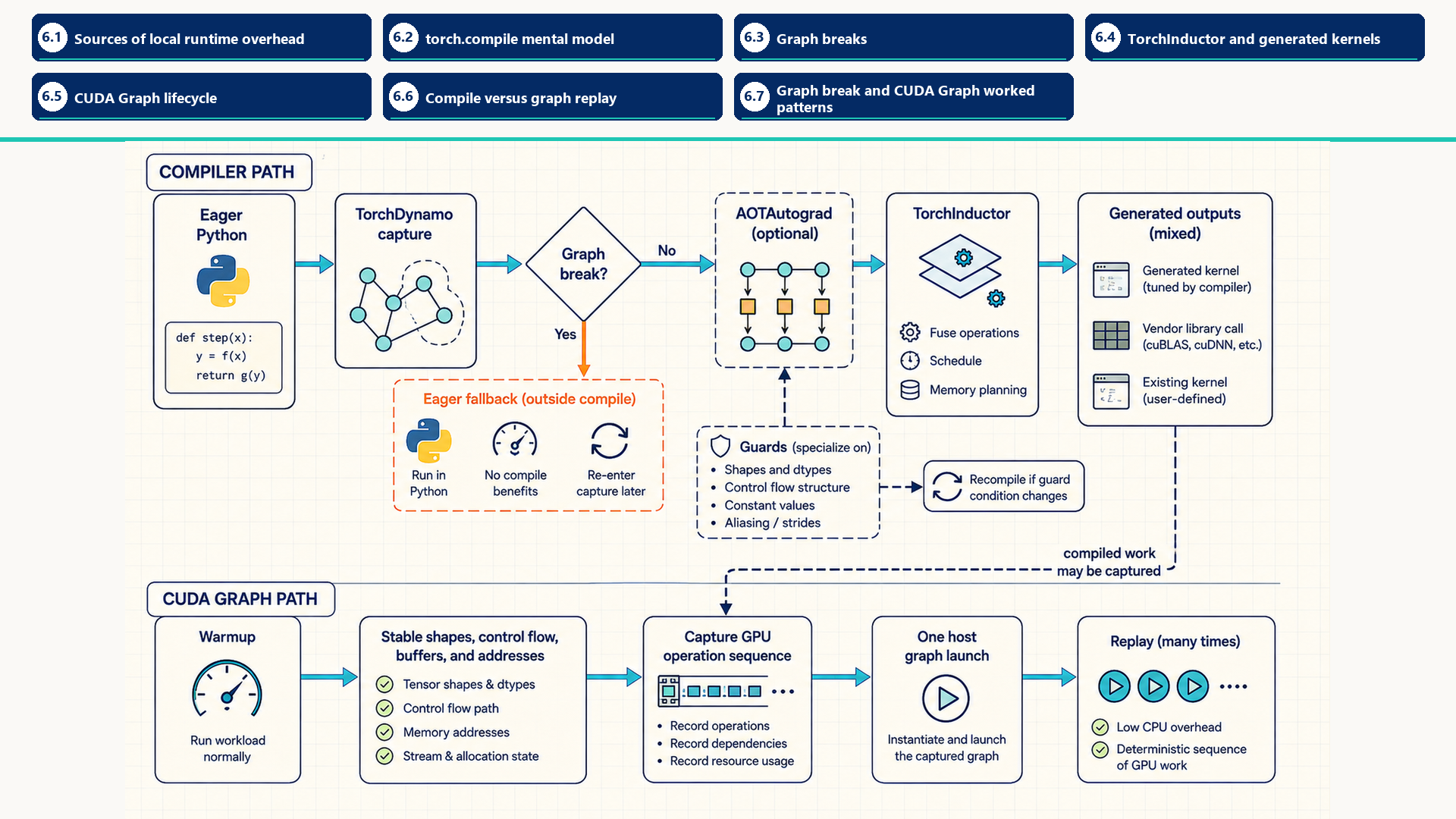
The compiler path shows TorchDynamo, optional AOTAutograd handling, TorchInductor, and mixed compiled or eager output. The CUDA Graph path requires warmup, stable shapes, control flow, buffers, and memory addresses before capture. Compiled work may later be captured, but a compiler graph and a CUDA Graph are not the same object.

The levers this chapter develops, in the vocabulary of Section 1.6.1, are cut fixed overhead, because capture and replay remove host work from every step, and move fewer bytes, because fusion removes intermediate tensors.

6.1 Sources of local runtime overhead

Single-worker runtime overhead is the cost paid inside one model-worker process while it executes a repeated model step. It includes Python dispatch through the PyTorch operator stack, compiler fallback to eager execution, kernel launch overhead, allocator churn, host-device synchronization, and small unfused GPU kernels.

A decode loop with many tiny kernels can remain slow even under a strong batching policy. The scheduler can admit more requests and share a model step’s launch cost across a batch, but the worker still has to launch and run that step. Later compiler and runtime techniques are useful when profiling shows that this cost, rather than request admission or KV-cache capacity, is the limiting factor.

• Python dispatch overhead: Time spent entering Python and the PyTorch dispatcher for many small operations. It is most visible when GPU kernels are short and repeated.
• Eager fallback regions: When compiler capture cannot cover a hot operation, that region runs through ordinary eager dispatch. Repeated fallback reduces fusion and can reintroduce Python overhead between compiled regions.
• Launch overhead: Fixed CPU-side cost of launching GPU work. It matters when each kernel does little work, such as small-batch decode or many elementwise operations.
• Allocator and copy overhead: Repeated temporary allocations or host-device transfers can dominate before the kernel math becomes the bottleneck.

Engine knobs cannot fully compensate for a local worker that launches too many tiny kernels, synchronizes with the host on every step, or recompiles constantly. Once the local model step is stable, batching, paging, and scheduling policies can be evaluated without confusing scheduler effects with per-worker runtime overhead.

6.2 torch.compile mental model

torch.compile is the PyTorch entry point for turning suitable eager PyTorch code into captured graph regions that can be optimized and lowered. The optimized object is the traceable runtime region of tensor operations reached from the Python program.

One word, three meanings: graph

Autograd graph: the record PyTorch builds during the forward pass of which operation produced which tensor, so that the backward pass can walk it and compute gradients (Section 1.5). It exists whenever gradients are required, with or without a compiler.

Compiler graph: the region of tensor operations that torch.compile captures so it can fuse, simplify, and lower them. Section 6.3 describes where capture stops. It can change which arithmetic runs.

CUDA Graph: a recorded sequence of already chosen GPU operations that is replayed with less host work (Section 6.5). It changes how the same work is launched, not what the work is.

• Eager execution: Default PyTorch mode where operations run one after another through the dispatcher. It is flexible, but many small operations can create CPU dispatch overhead and extra intermediate tensors in HBM.
• Graph capture: The compiler records a region of tensor operations when Python control flow, operators, and shapes are traceable enough.
• Graph optimization: The compiler can fuse compatible operations, remove unnecessary intermediates, and choose generated kernels for a captured region.
• Lowering: The optimized graph is translated into executable code. In many PyTorch paths, TorchInductor emits Triton or other backend code for fused regions.
• Guard: A condition recorded for a compiled region, such as an input type, shape property, or Python value. When a guard no longer holds, PyTorch may compile another variant or run a different path.
• Graph break: A boundary where TorchDynamo cannot keep execution in one captured region, so one function becomes several compiled and eager pieces (Section 6.3).

The PyTorch compiler path begins at Python execution rather than at Triton, and the three components below carry a captured region from Python frames to executable code³. Chapter 4’s Triton pipeline is one possible generated-kernel path, not a diagram of this complete stack.

Definition - Compiler stack terms

TorchDynamo: Captures Python-level PyTorch execution into graph regions when control flow and operators are traceable.

AOTAutograd: Stages forward and backward graphs for differentiable computation when gradients are involved.

TorchInductor: Lowers captured graphs into executable optimized code, often emitting Triton kernels for fused regions.

Common torch.compile settings

mode='default': Balanced compile behavior. Use it first when you want compiler benefits without aggressively changing overhead or autotuning behavior.

mode='reduce-overhead': Targets Python and launch overhead, often by using CUDA Graphs where the graph is safe⁴. It can increase memory use because reusable workspaces or graph state may be cached.

mode='max-autotune': Allows more autotuning and can use Triton or template-based matrix multiplication paths on supported devices. It may improve steady-state speed at the cost of compilation/autotuning time.

dynamic=True or dynamic=False: Controls dynamic-shape tracing policy. Dynamic kernels can reduce recompilation for varying shapes, but some operations still force specialization.

torch.compile and @triton.jit are different entry points. torch.compile starts from PyTorch model code and tries to capture graph regions before lowering them. @triton.jit starts from an explicitly written Triton kernel function and compiles that tile program. A torch.compile path may generate Triton kernels internally, but that does not make hand-written Triton code the same object as a compiled PyTorch graph.

6.3 Graph breaks

A graph break splits a Python function around code that TorchDynamo cannot represent in the current graph. It ends one captured region, runs the unsupported code eagerly, and may resume capture afterward. The performance cost depends on where and how often this happens: a break during one-time setup may not matter, while a break in every decode step can restore Python dispatch, block fusion across the boundary, or synchronize a tensor value with the host.

Breaks usually arise when tensor execution crosses into Python values, unsupported effects, or unstable specialization. The following cases separate those causes so diagnostics can target the actual boundary.

• Scalar extraction: Calls such as .item() move a tensor value into Python and commonly force GPU-to-CPU synchronization or a graph break. Some releases and configurations can capture scalar outputs, so diagnostics must confirm the observed path.
• Data-dependent Python branches: Python if or loop decisions based on tensor values cannot usually be traced as a single static graph.
• Unsupported operations: An operator, mutation pattern, or side effect can cause a graph break when TorchDynamo cannot capture it. Under default partial-graph compilation that region can run eagerly. An operation captured successfully but unsupported by the selected backend can instead cause a compilation error. Fallback is not guaranteed.
• Dynamic shape churn: Frequent shape changes can cause recompilation or guards that prevent a stable compiled path. A failed shape guard requests another compiled variant. That is distinct from a graph break inside a captured function.
• Host I/O in hot paths: Printing, logging tensor values, or debugging inside a repeated GPU path can force synchronization and graph breaks.

After locating the breaks, inspect the captured regions to see which kernels TorchInductor generated, what it fused, and how much memory traffic remains.

6.4 TorchInductor and generated kernels

TorchInductor is the PyTorch compiler backend that lowers captured graph regions into executable code. In many CUDA paths it emits generated Triton kernels for fused regions and calls vendor libraries or existing kernels for operations that are better handled by those libraries.

• Captured graph: The traceable tensor program handed to the backend after TorchDynamo and, when needed, AOTAutograd have staged the computation.
• Fusion: Combining compatible operations so an intermediate may remain in registers or shared memory, be recomputed cheaply, or avoid a separate HBM write and read. Exact placement depends on compiler decisions and resource limits.
• Generated kernel: Kernel code emitted by the compiler for a specific graph region, dtype, layout, and shape family. Generated does not mean universally optimal. It means specialized to the compiler’s view of the program.
• Scheduler and lowering: Compiler decisions that choose loop structure, tiling, vectorization, memory access order, and which operations remain separate calls.
• Limits: Poor algorithmic structure, unsupported operators, dynamic control flow, request scheduling, cache paging, and cross-rank communication are outside what TorchInductor can fix by itself.

The main performance win is reducing unnecessary HBM traffic and launch count. For example, a chain of elementwise operations may become one generated kernel that reads input once, keeps temporary values in registers, and writes the final result once. That is a different kind of win from CUDA Graph replay, which keeps the same kernels but launches them with less CPU overhead.

When generated kernels are slow, first inspect the source graph and shape assumptions. A compiler backend can improve locality through fusion, scheduling, and layout choices, but those transformations are limited by the operations and dependencies in the source graph. It does not by itself turn request-dependent host control flow into a static batching policy.

The number of generated Triton kernels is not fixed. It is a property of one compiled run: graph regions, shapes, dtypes, layouts, dynamic-shape guards, and autotuning choices determine how many kernels are emitted. Count them from compiler logs, profiler traces, or the TorchInductor/Triton cache for the specific workload, not from a static catalog.

Generated-kernel caveat

Generated Triton is often the right outcome for fused elementwise and reduction regions, but vendor libraries can still be better for standard GEMMs, convolutions, and collectives. The compiler backend chooses among generated kernels, templates, and library calls. Performance work should inspect the chosen path before replacing it by hand.

Generated code is useful only when the selected kernel path reduces measured launch count or memory traffic for the actual shapes. Generation alone does not make it faster than a vendor kernel. The next question is whether the remaining delay comes from kernel execution or from repeatedly launching an otherwise stable sequence.

6.5 CUDA Graph lifecycle

A CUDA Graph is a recorded sequence of GPU operations that can be replayed with much lower CPU launch overhead than issuing each kernel separately⁵. Replay preserves the recorded kernel computation. Its main benefit is reducing repeated host-side launch and dispatch cost for a stable sequence of work.

The mechanism has three phases. Warmup runs first so kernels, autotuning, and allocator state are initialized. Capture records the steady sequence of operations and their memory addresses. Replay launches that captured sequence again after new inputs have been copied into the same static buffers.

The timeline compares separate host launches with one graph launch of the same device operations. Graph construction appears before the graph-launch example. Warmup and input-buffer preparation are not drawn.

Figure 6.2: One graph launch submits the recorded device operations with less host launch work (Lecture 2, slide 80).

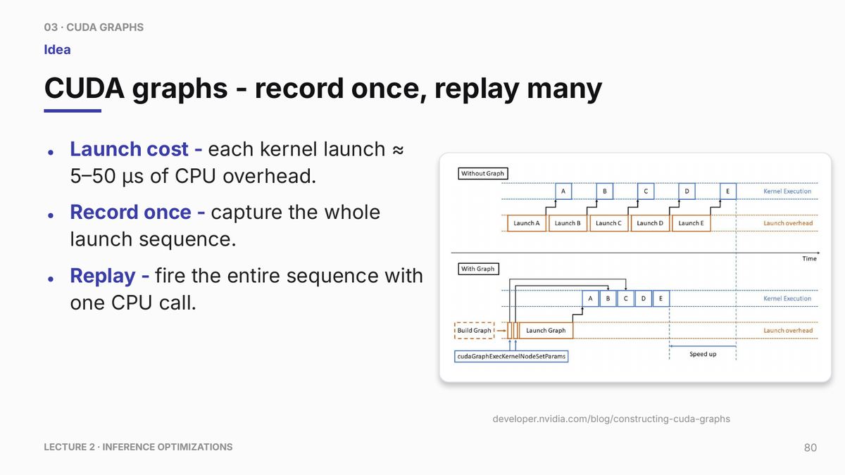
Warmup completes lazy initialization, autotuning, and allocations. Capture records supported operations and dependencies against stable virtual addresses and stream-capture rules⁶. One replay is one graph-launch submission containing the recorded device operations, not one fused device kernel.

Chart note

Measured or compared: Separate launches of five illustrative kernels versus one graph launch containing those same kernels.

Axes, units, and series: Horizontal position indicates execution order. Separate lanes show host launch work and GPU kernels. The slide includes an approximate per-launch overhead range, but it is not a measurement of this chapter’s workload.

Interpretation: The device still executes the recorded kernels. The shorter host path illustrates reduced submission overhead, not kernel fusion. Warmup and capture belong outside steady-state timing, although this figure does not show the complete preparation process.

Source status: Course-slide schematic. Its timing range and drawn speedup are not hardware-independent guarantees. The worked recipe below requires a measurement of the actual workload.

The main constraint is stability. Shapes, control flow, and memory addresses must remain compatible with the captured graph. If every request changes tensor shape or allocates new buffers, CUDA Graph replay either fails or loses most of its value.

• Dynamic-shape failure: If each replay-sized region receives new sequence lengths, batch sizes, or tensor layouts, the compiler may recompile and CUDA Graph capture may no longer match the new execution path.
• Address stability: A captured graph reuses the same pointer arguments. Copy new request data into the static buffers whose addresses were recorded during capture.
• Control-flow failure: Data-dependent Python branches or request-dependent operator sequences can make the captured graph represent only one path while production takes many paths.
• Allocation failure: Allocations during capture can bake allocator behavior into the graph or cause capture errors. Warmup and pre-allocation keep steady-state memory addresses predictable.

This is why serving systems often bucket shapes or pre-allocate decode buffers before using graph replay. Shape bucketing preserves enough regularity for compilation and replay, while the scheduler still handles variable request lengths at a coarser level.

6.6 Compile versus graph replay

Compilation and graph replay are different runtime changes. Compilation transforms captured computation and may generate new fused kernels. CUDA Graph replay records an already-selected sequence of GPU work and relaunches it with lower CPU overhead.

• Compilation fit: The hot path contains many traceable tensor operations that can be fused, simplified, or lowered into better kernels.
• CUDA Graph replay fit: The hot path already has acceptable kernels but repeated launches and Python dispatch dominate wall time.
• Combined fit: A compiled steady-state region can be captured with stable shapes and stable memory addresses.
• Eager-execution fit: Shapes, control flow, memory addresses, or request membership change too frequently for stable capture, or profiling shows that capture overhead is outside the limiting path.

The comparison below separates compiler graphs, which can transform computation, from CUDA Graph replay, which relaunches an already selected sequence.

The structured comparison below turns that distinction into a selection rule: transformation changes the computation, replay changes how an existing operation sequence is submitted, and the combined path requires both capture compatibility and worthwhile compiler output.

Table 6.1: torch.compile versus CUDA Graphs.

Mechanism	Changes computation?	Primary benefit	Main constraint
torch.compile	Yes, can fuse and generate kernels	May reduce Python overhead, launch count, and intermediate memory traffic	Graph breaks, unsupported ops, recompilation
CUDA Graphs	No, replays captured work	Reduces CPU launch overhead	Static shapes and stable memory addresses
Combined	Compile first, then replay stable work	Reduced kernel count or memory traffic with lower host launch overhead	Harder debugging and stricter shape discipline

The operational sequence is usually compile first, then capture only the stable steady-state path. Capturing before compilation can preserve too many small kernels. Compiling without checking graph breaks can leave eager gaps that still dominate the loop.

6.7 Graph break and CUDA Graph worked patterns

A common local-runtime repair sequence has three stages. First, make the hot function traceable enough that torch.compile can capture it. Second, stabilize input shapes and memory addresses enough that CUDA Graph replay can remove repeated launch overhead. Third, measure the steady-state path separately from warmup, compilation, and allocation.

• Trace repair: The hot tensor path excludes Python-side scalar extraction, host I/O, and data-dependent branches.
• Static buffers: Pre-allocated tensors whose memory addresses are reused across CUDA Graph replays.
• Warmup isolation: Compilation, kernel autotuning, and allocator initialization occur before capture so the captured sequence represents steady-state work.
• Replay validation: Valid replay copies new inputs into the captured buffers and copies or clones outputs before the next replay overwrites them.

6.7.1 Resolving graph breaks in RMS-normalization

This toy normalization loop places four capture problems in one short example: scalar extraction that can synchronize a GPU value with the CPU, a Python branch on that extracted value, host logging in the repeated path, and tensor operations that must remain traceable. The same patterns can occur in many model operations, not only normalization.

The optimization principle is to keep decisions in tensor space when they belong on the GPU and to keep host-side diagnostics out of the repeated compiled region. The two functions below must preserve the returned feature tensor and updated buffer within a numerical tolerance. Console printing is deliberately excluded from that equivalence contract.

The functions are an abbreviated inference toy. h is a batch of feature rows with shape (B, D), where B and D are positive. state is a same-shaped illustrative running buffer: each call retains 90 percent of its previous value and adds 10 percent of the current returned features. Both inputs are finite FP32 tensors on the same device, with values small enough that squaring and reduction stay finite. This example uses (2, 16) contiguous tensors, no gradients, and either CPU for arithmetic validation or CUDA for the capture investigation. Both outputs have the same shape, dtype, and device as the inputs. Neither input is modified in place.

Root-mean-square (RMS) normalization divides each feature by the square root of its row’s mean squared value. The code adds epsilon = 1e-6 inside that square root so a zero row has a nonzero denominator. mean(dim=-1, keepdim=True) produces shape (B, 1), which broadcasts across the D features of each row. This is the RMS operation with no learned affine weights⁷. The later threshold and running-buffer update are choices of this toy, not parts of standard RMS normalization.

After normalization, scale = h.abs().max() is one scalar over the whole batch. If it exceeds 3, every row is divided by that scalar. Otherwise, every row is retained. This is a batch-wide decision, not a separate branch per row. The update uses the features after this decision and returns a new state tensor.

Worked example: Resolving graph breaks in RMS-normalization

The first function contains patterns that commonly create synchronization and graph breaks. The second keeps the decision in tensor operations so the current compiler has a better chance of capturing the hot region. Graph-break diagnostics must confirm the result for the installed PyTorch release. Calling .item() extracts a tensor value as a Python scalar, forcing a GPU-to-CPU synchronization that stalls execution. Python if conditions on tensor values break compilation. torch.where expresses selection in tensor form. Clamping the denominator prevents a zero-scale input from creating invalid values or gradients in the unselected division branch. Printing tensor values in a hot loop can synchronize or break capture.

Broken version. The first function extracts a GPU value into Python and branches on it.

Revised version. The second function keeps the data-dependent choice in tensor operations.

Validation inputs and expected results. Two rows of sixteen ones give a normalized maximum near 1, so the false branch retains their values near 1. Two rows [4, 0, ..., 0] have mean square 16/16 = 1, so their normalized maximum is near 4. The true branch divides by that maximum and returns rows [1, 0, ..., 0]. Starting from state = 0.25 in every position, the latter update gives 0.9*0.25 + 0.1*1 = 0.325 at the first coordinate and 0.225 elsewhere. A zero-input case also checks that the unselected division stays finite and that the new state is 0.225 throughout. These are calculated expectations, not timing results.

The invocation below checks both returned tensors against the original function on all three inputs outside timing. It also checks the branch condition, finite outputs, the explicit running-buffer rule, and unchanged inputs. The numerical tolerances apply to these FP32 examples. Passing them does not establish gradient equivalence, compiler capture, or a speedup.

Code example: Resolving graph breaks in RMS-normalization

import torch

def broken_normalize_step(h: torch.Tensor, state: torch.Tensor):
    h = h * torch.rsqrt(h.pow(2).mean(dim=-1, keepdim=True) + 1e-6)
    scale = h.abs().max().item()  # Extracts a host scalar on CUDA.
    if scale > 3.0:
        h = h / scale
    print(f"max|h| = {scale:.3f}")
    state = 0.9 * state + 0.1 * h
    return h, state

def fixed_normalize_step(h: torch.Tensor, state: torch.Tensor):
    h = h * torch.rsqrt(h.pow(2).mean(dim=-1, keepdim=True) + 1e-6)
    scale = h.abs().max()
    # Both candidate tensors are computed, including the unselected one.
    safe_scale = scale.clamp_min(torch.finfo(h.dtype).tiny)
    h = torch.where(scale > 3.0, h / safe_scale, h)
    state = 0.9 * state + 0.1 * h
    return h, state

# Arithmetic validation only, outside compilation and timing.
device = torch.device("cpu")
dense = torch.ones((2, 16), device=device, dtype=torch.float32)
sparse = torch.zeros_like(dense)
sparse[:, 0] = 4.0
cases = [("below", dense, False), ("above", sparse, True),
         ("zero", torch.zeros_like(dense), False)]
with torch.inference_mode():
    for label, h_in, expected_branch in cases:
        state_in = torch.full_like(h_in, 0.25)
        h_before, state_before = h_in.clone(), state_in.clone()
        normalized = h_in * torch.rsqrt(
            h_in.square().mean(dim=-1, keepdim=True) + 1e-6
        )
        assert bool(normalized.abs().max() > 3.0) == expected_branch
        ref_h, ref_state = broken_normalize_step(h_in, state_in)
        got_h, got_state = fixed_normalize_step(h_in, state_in)
        for actual, reference in [(got_h, ref_h), (got_state, ref_state)]:
            assert actual.shape == h_in.shape
            assert actual.dtype == h_in.dtype and actual.device == h_in.device
            assert bool(torch.isfinite(actual).all())
            torch.testing.assert_close(actual, reference, rtol=1e-5, atol=1e-6)
        expected_h = normalized if not expected_branch else h_in / 4.0
        torch.testing.assert_close(got_h, expected_h, rtol=1e-5, atol=1e-6)
        torch.testing.assert_close(
            got_state, 0.9 * state_in + 0.1 * got_h, rtol=1e-5, atol=1e-6
        )
        assert torch.equal(h_in, h_before) and torch.equal(state_in, state_before)
        print(label, "feature and state checks passed")

Replacing the host-side condition with torch.where keeps the selection in tensor form and avoids extracting scale into Python. That change can preserve a captured region, but it does not guarantee one fused kernel: compiler diagnostics and a profiler trace must show which regions and kernels were produced.

6.7.2 Manual CUDA Graph capture and replay recipe

torch.compile(mode='reduce-overhead') can use CUDA Graphs for eligible regions, but CUDA Graph capture is not available to every workload⁸. Manual capture is useful when an engineer needs direct control over buffers and stream dependencies. Inputs and outputs use stable addresses, and warmup must complete lazy initialization, autotuning, and allocations before capture. A side-stream warmup is a robust pattern when its dependencies are synchronized correctly.

Worked example: Manual CUDA Graph capture and replay recipe

This recipe shows the manual capture of a module using static buffers, a side-stream warmup to isolate pending events, and replay with output cloning. CUDA Graphs capture operations bound to exact memory addresses, requiring fixed, static input/output buffers. model.eval() selects evaluation behavior and torch.inference_mode() disables autograd bookkeeping. These are recommended settings for inference, but not actual CUDA Graph capture requirements, as capture can also be used for training steps. A synchronized side-stream warmup is a robust way to isolate initialization and allocations before capture. Calling graph.replay() submits the recorded sequence without repeating Python dispatch for every captured operation. The replay helper documents its intended input shape, device, and dtype, and rejects unintended broadcasting before copying. A clone of static_out is needed only when the caller preserves that result across a later replay. The final check compares the replay result with an eager reference outside the timed path. Cloning and the correctness check add work outside the graph.

This helper assumes ordered calls on one CUDA stream. Its shared static_in and static_out buffers are not safe for overlapping requests from independent streams or host threads. Concurrent serving needs separate buffer/graph instances or explicit serialization through completion of the input copy, replay, and output clone.⁹

Code example: Manual CUDA Graph capture and replay recipe

import torch

# Target module to graph (e.g. a small MLP layer)
model = torch.nn.Linear(256, 256).cuda().eval()
example_input = torch.randn(1, 256, device="cuda")

# Step 1: Create static input/output buffers
static_in = example_input.clone()

with torch.inference_mode():
    # Step 2: Warmup on a dedicated CUDA stream
    # This isolates compilation/allocations from the default stream
    warmup_stream = torch.cuda.Stream()
    warmup_stream.wait_stream(torch.cuda.current_stream())
    with torch.cuda.stream(warmup_stream):
        for _ in range(10):
            static_out = model(static_in)
    torch.cuda.current_stream().wait_stream(warmup_stream)

    # Step 3: Record the graph on PyTorch's capture stream
    graph = torch.cuda.CUDAGraph()
    with torch.cuda.graph(graph):
        static_out = model(static_in)

# Step 4: Replay function for new inputs
@torch.inference_mode()
def run_graphed_inference(x):
    # Reject unintended broadcasting or shape/device/dtype mismatches
    if x.shape != static_in.shape or x.dtype != static_in.dtype or x.device != static_in.device:
        raise ValueError("Input must match the captured static_in shape, dtype, and device.")
    # Copy new data into the captured memory address
    static_in.copy_(x)
    graph.replay()
    # Clone output to prevent subsequent runs from overwriting it
    return static_out.clone()

# Step 5: Check replay against eager output outside the timed path
validation_input = torch.randn_like(example_input)
with torch.inference_mode():
    eager_output = model(validation_input)
replay_output = run_graphed_inference(validation_input)
torch.testing.assert_close(replay_output, eager_output, rtol=1e-5, atol=1e-6)

During capture, PyTorch records supported CUDA operations and their dependencies against the graph’s memory addresses. Each call copies new values into static_in and submits the recorded graph through one graph launch, while the recorded kernels remain separate device operations unless compilation fused them earlier. static_out is reused, so cloning is conditional on whether a result must survive the next replay.

Compilation is justified when captured operations can be simplified, fused, or lowered more effectively. CUDA Graph replay is justified when a stable sequence already has suitable kernels but host launch work remains visible. The evidence separates compile and warmup cost, compares eager and optimized outputs, and establishes whether steady-state end-to-end time improved.

These runtime methods apply to both training and inference, but the useful capture boundary depends on which state changes during the workload. Chapter 7 makes those lifetimes concrete by following parameters, activations, gradients, optimizer state, input delivery, and precision through one training step.

---

1. Ansel, J., et al. (2024). PyTorch 2: Faster Machine Learning Through Dynamic Python Bytecode Transformation and Graph Compilation. In Proceedings of ASPLOS 2024. https://doi.org/10.1145/3620665.3640366. Supports that TorchDynamo captures Python bytecode into FX graphs and that TorchInductor is the default backend lowering to Triton on GPU and C++ on CPU. Limit: reported speedups are A100 geometric means over the paper benchmark suite, not guarantees for the chapter toy shapes.

2. PyTorch. (2.14 documentation). torch.compile. https://docs.pytorch.org/docs/2.14/generated/torch.compile.html. Supports that reduce-overhead lowers Python overhead with CUDA graphs for eligible CUDA only graphs without input mutation, that extra workspace caching can raise memory use, and that coverage is not guaranteed. Limit: eligible behavior and debug flags depend on the installed release; the chapter keeps mode selection as a measurement decision.

3. Ansel, J., et al. (2024). PyTorch 2: Faster Machine Learning Through Dynamic Python Bytecode Transformation and Graph Compilation. In Proceedings of ASPLOS 2024. https://doi.org/10.1145/3620665.3640366. Supports that TorchDynamo captures Python bytecode into FX graphs and that TorchInductor is the default backend lowering to Triton on GPU and C++ on CPU. Limit: reported speedups are A100 geometric means over the paper benchmark suite, not guarantees for the chapter toy shapes.

4. PyTorch. (2.14 documentation). torch.compile. https://docs.pytorch.org/docs/2.14/generated/torch.compile.html. Supports that reduce-overhead lowers Python overhead with CUDA graphs for eligible CUDA only graphs without input mutation, that extra workspace caching can raise memory use, and that coverage is not guaranteed. Limit: eligible behavior and debug flags depend on the installed release; the chapter keeps mode selection as a measurement decision.

5. NVIDIA. (2024, March 5). CUDA C++ Programming Guide 12.4: CUDA Graphs. https://docs.nvidia.com/cuda/archive/12.4.0/cuda-c-programming-guide/index.html#cuda-graphs. Supports stream capture with cudaStreamBeginCapture and cudaStreamEndCapture, same stream begin and end rules, fixed argument and address requirements, and replay as one launch of the recorded sequence. Limit: the guide describes the CUDA API path; PyTorch adds its own eligibility and partitioning rules on top.

6. NVIDIA. (2024, March 5). CUDA C++ Programming Guide 12.4: CUDA Graphs. https://docs.nvidia.com/cuda/archive/12.4.0/cuda-c-programming-guide/index.html#cuda-graphs. Supports stream capture with cudaStreamBeginCapture and cudaStreamEndCapture, same stream begin and end rules, fixed argument and address requirements, and replay as one launch of the recorded sequence. Limit: the guide describes the CUDA API path; PyTorch adds its own eligibility and partitioning rules on top.

7. PyTorch. (2.14 documentation). RMSNorm. Official documentation. Supports normalization by the square root of mean squares plus epsilon over the selected final dimensions. Limit: the toy uses an explicit epsilon and no learned affine weights. Its threshold and running buffer are illustrative additions, not the library layer’s contract.

8. PyTorch. (2.14 documentation). torch.compile. https://docs.pytorch.org/docs/2.14/generated/torch.compile.html. Supports that reduce-overhead lowers Python overhead with CUDA graphs for eligible CUDA only graphs without input mutation, that extra workspace caching can raise memory use, and that coverage is not guaranteed. Limit: eligible behavior and debug flags depend on the installed release; the chapter keeps mode selection as a measurement decision.

9. PyTorch. (2.14 documentation). CUDA semantics: CUDA graphs. CUDA graph usage and constraints. Describes static replay addresses, stream ordering, and private graph memory pools. The serialization requirement for this example follows from its shared input and output buffers.