3  Software to CUDA

Connect framework calls and settings to CUDA launches, streams, memory transfers, and the software layer that owns each control.

When a single PyTorch model call launches hundreds of kernels, the gap between GPU computation and host dispatch can dominate execution time. Small decode steps may wait on launch overhead, and uncoalesced memory reads can stall bandwidth before the GPU reaches its arithmetic limits.

Compute Unified Device Architecture (CUDA) is the programming model and platform beneath most NVIDIA GPU deep learning work. A Python program may call PyTorch, a compiler may emit Triton, and a serving engine may hide scheduling details, but the GPU still executes kernels over grids, blocks, threads, and warps. Section 3.2 develops that hierarchy, and Section 3.3 the memory and transfer model that goes with it.

A single PyTorch statement such as logits = model(input_ids) expands into many kernel launches in one forward pass, whether training or inference. A one-token decode step can also launch many small kernels. Compilation, fusion, batching, or CUDA Graph replay can reduce the exposed launch work when the path meets the technique’s static-shape and control-flow requirements. Chapter 6 develops capture, warmup, and graph-break limits.

To locate a delay, identify which tensor, backend, or stream setting selects the downstream kernel or copy, then inspect the profiler event that connects it to the end metric.

The layer map below traces effects rather than assigning an exclusive owner. Model code shapes inputs and operations. PyTorch interprets tensor and backend settings. Compilers and libraries turn those choices into kernels. CUDA orders their submission. Serving or distributed runtimes coordinate work around each execution. A change at one layer can alter work observed at later layers, so the immediate action and downstream result are recorded together.

• Model and application layer: Defines model calls, input preparation, generation behavior, and the performance question being measured.
• PyTorch framework layer: Stores tensor metadata and provides autograd, device placement, dispatch, the caching allocator, and framework-level measurement interfaces.
• Compiler and kernel layer: Turns operations into vendor, generated, Triton, or CUDA kernels and controls the layout, tiling, fusion, and load/store behavior of hot GPU work.
• CUDA runtime and library layer: Provides device contexts, streams, events, copies, launch ordering, and access to vendor libraries such as cuBLAS or cuDNN.
• Serving and distributed layer: Schedules request admission and KV-cache use, and coordinates process groups, collective requests, and rank placement around one model execution path.

Saying that state is “local” requires naming the boundary, because physical location and software ownership differ. HBM, for example, is GPU-attached device memory: close to the GPU but not on-chip storage. The remaining chapters use four scopes:

• On-chip: Registers and shared memory inside one SM, plus the device-wide L2 cache on the GPU die.
• Same-GPU: L2 cache and HBM, visible to every SM on the device. L2 is also on-chip, while HBM is off-chip.
• Same-server: GPUs and host memory joined by intra-node links such as PCIe or NVLink.
• Process- or rank-local: Software ownership: which process or distributed rank holds and manages the object.

A framework dispatches a vendor-library operation or a custom kernel. The library or launcher uses CUDA runtime or driver APIs to submit the resulting GPU work to a stream queue.

Figure 3.1: Framework operations become ordered CUDA work before GPU threads execute them.

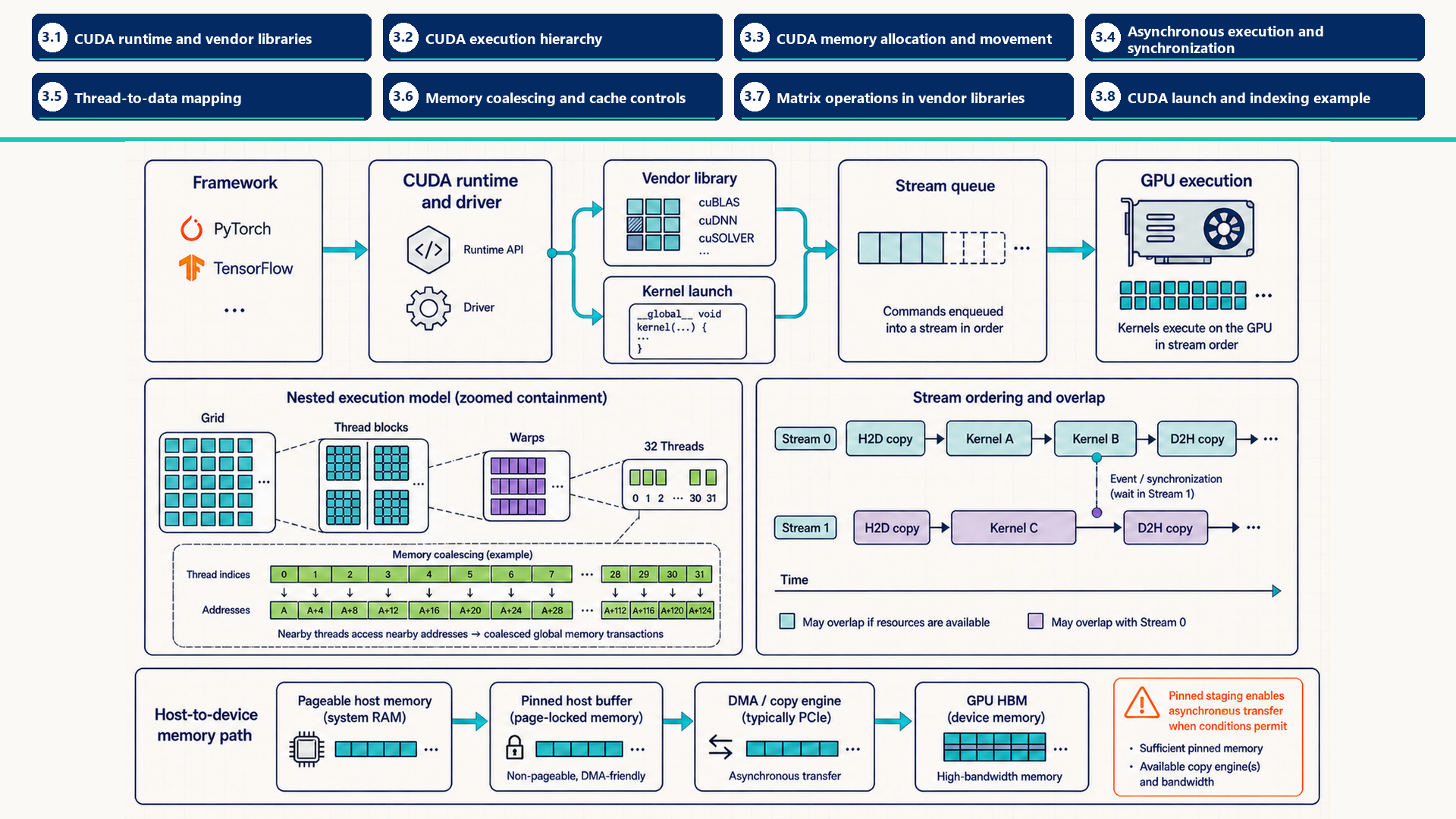
The upper path separates host dispatch from GPU execution. The middle panels show grid, block, warp, and thread containment, nearby-address access within a warp, and ordering or synchronization across streams. The lower path shows ordinary host data staged through pinned memory and transferred by a copy engine, typically over PCI Express (PCIe), into GPU HBM.

The levers this chapter develops, in the vocabulary of Section 1.6.1, are cut fixed overhead through fewer and cheaper launches, move fewer bytes through coalesced access, and keep the hardware busy through streams and overlap.

3.1 CUDA runtime and vendor libraries

Hundreds of launches in one model call must pass through a host-side layer before the GPU can perform useful work. The CUDA software layer provides those APIs between framework code and NVIDIA GPU execution. Every kernel launch, explicit copy, stream dependency, event, and vendor-library call passes through the runtime or driver path.

3.1.1 Runtime and device context

The runtime submits host API requests, the driver loads and launches executable GPU code, and the device context holds process-visible execution state. Their versions and context state determine whether compiled kernels and libraries can execute on the selected GPU.

• CUDA runtime: The host API for selecting devices, allocating memory, launching kernels, creating streams and events, copying memory, and synchronizing work.
• CUDA driver: The lower-level interface that loads executable GPU code, manages device interaction, and links runtime requests to GPU execution through the installed kernel driver.
• Device context: The process-visible execution state for a GPU, including loaded modules, allocations, streams, and runtime resources.
• Framework boundary: PyTorch exposes many runtime operations through torch.cuda. The framework still defines tensor behavior and dispatch policy.

CUDA Graphs also use this submission layer, but Chapter 6 gives their full warmup, capture, replay, and graph-break sequence after ordinary launches are defined.

3.1.2 Vendor kernel libraries

Vendor libraries supply prebuilt optimized kernels behind stable APIs. The application or framework launches these operations over GPU tensors instead of editing the underlying kernel source.

• cuBLAS and cuBLASLt: NVIDIA matrix and linear-algebra libraries. Transformer projections commonly reach their tensor-core GEMM implementations when dimensions, dtype, layout, and alignment are supported.
• cuDNN: NVIDIA neural-network operator library, especially important for convolution-oriented workloads and other supported primitives.
• Vendor library kernel: A compiled GPU implementation selected through a library API. It provides the baseline that a custom CUDA or Triton kernel should beat on the measured workload.
• Communication boundary: NVIDIA Collective Communications Library (NCCL) is also a vendor library, but its collectives require processes, ranks, process groups, and physical fabrics. Chapter 12 develops that communication stack.

Vendor libraries are the default when a supported operation already has a tuned kernel. Custom code is justified only after that baseline is measured on the real shapes and data type. The next question is how CUDA divides any selected kernel into grids, blocks, warps, and threads when it executes.

3.2 CUDA execution hierarchy

CUDA execution objects appear in the order a program encounters them. The host is the CPU-side program. The device is the GPU. A kernel is launched from the host onto the device, and the launch creates a grid of blocks, each containing threads grouped for scheduling into warps.

The CUDA execution hierarchy should be read from the launch boundary down to the scheduling unit. Each level answers a different question: who launches work, where it runs, how work is grouped, and which threads execute together.

The hierarchy is logical, not a permanent one-to-one wiring to physical units. One kernel launch creates a grid. The grid contains blocks. An available Streaming Multiprocessor (SM) admits a block when resources permit. Warp schedulers issue active lanes from the block’s warps. A thread is one logical lane rather than a CUDA core reserved for that thread.

• Host: The CPU-side program that allocates tensors, launches kernels, schedules framework work, and may synchronize with the GPU. Python code normally runs on the host even when tensors live on the device.
• Device: The GPU selected for execution. A process may see multiple devices, but each device has its own SMs, HBM, streams, and allocator state.
• Kernel: The GPU function introduced in Section 2.2. A PyTorch operation can launch one kernel, many kernels, or a fused/generated kernel depending on the backend path.
• Grid: The complete set of blocks created by one kernel launch. Grid dimensions describe how much independent block-level work is exposed.
• Block / CTA: The cooperating thread group introduced in Section 2.2. On NVIDIA GPUs, a block is assigned to one SM for execution. A single block does not span multiple SMs.
• Thread: The logical scalar worker that has registers and computes one or more data elements according to the kernel’s index mapping.
• Warp: The 32-thread scheduling group introduced in Section 2.2. Warps explain why adjacent lane access, branch divergence, and coalescing matter.

These objects describe where CUDA work is placed. The next terms describe how efficiently resident warps use execution lanes and hide long-latency operations.

• Warp divergence: A warp diverges when lanes in the same warp must follow different control-flow paths. The hardware serializes the paths under masks, so useful lane utilization drops even though the kernel is logically correct.
• Predication: A compiler or hardware technique that can execute short conditional work under lane masks instead of taking a full branch. It can reduce branch overhead, but both paths may still consume instructions.
• Occupancy: As defined in Section 2.2, the ratio of active resident warps on an SM to the maximum possible resident warps. It is useful because other warps can run while one warp waits on memory, but high occupancy is not the same as high throughput.
• Latency hiding: The SM scheduler keeps execution units busy by switching to ready warps when one warp stalls on HBM, dependencies, or synchronization. If too few warps are resident, long HBM latency becomes visible as idle cycles.

Warp scheduling is the SM-level answer to HBM latency. A global-memory load can take far longer than an arithmetic instruction, so the SM relies on many resident warps to cover the wait. Register pressure, shared-memory use, large blocks, and launch shape can reduce resident warps. The optimization target is enough ready work to hide stalls while keeping memory accesses coalesced and instruction dependencies short.

Distinguishing execution limits

Divergence reduces useful lanes inside a warp. Low occupancy leaves too little ready work to cover latency. Poor coalescing expands the memory transactions needed for a warp’s data. A trace can show more than one limit, and each points to a different fix.

Divergence, low occupancy, and poor coalescing waste different resources, so a profiler must identify which limit is active before the launch is changed. This execution model assumes that tensors are available to the device. The next question is how memory is allocated and how bytes reach the kernel.

3.3 CUDA memory allocation and movement

Allocation and movement are part of the performance model, not background bookkeeping. A program can be mathematically correct and still slow or unstable because it allocates unpredictably, fragments memory, or synchronizes copies.

3.3.1 Host-device and peer-transfer ownership

Explicit transfers are initiated by framework placement calls or CUDA runtime APIs and executed over the path available between the source and destination. The list identifies the objects and hardware conditions that govern those transfers.

• Pinned host memory: Defined in Section 2.6. It is commonly used by DataLoaders and asynchronous copies, but pinning too much host memory leaves the operating system less it can move or page out.
• Asynchronous copy and streams: A copy can overlap with compute only when the copy is issued asynchronously, the host memory path supports it, and stream dependencies do not serialize the work. A later synchronization can still expose the full cost.
• cudaMemcpy: The CUDA runtime copy operation used to move bytes between host and device or between devices. In PyTorch this is usually hidden behind .to(device), .cuda(), .cpu(), or tensor copy calls.
• Direct Memory Access (DMA): Defined in Section 2.6. Pinned host memory is what makes a DMA-based GPU transfer possible without an intermediate copy, and the transfer still consumes interconnect bandwidth.
• PCIe transfer: Host-device or some device-device traffic over the PCIe bus. Its bandwidth is far below HBM, so repeated round trips should be avoided.
• Peer transfer: A GPU-to-GPU copy that can avoid host staging when peer access, topology, and the runtime configuration permit a direct path.
• Mapped host memory: Lets a GPU kernel access a host allocation through the system interconnect, which can be useful for small or irregular control data and slow for bulk tensor traffic.
• Managed memory: Can migrate or prefetch pages between processors. cudaMemAdvise and cudaMemPrefetchAsync guide residency, while ordinary L1 and L2 cache behavior remains hardware-managed.

A low-level CUDA lifecycle makes the hidden costs visible: allocate device memory, copy inputs from host to device, launch the kernel, synchronize only when required, copy results back if the host needs them, and free or reuse device memory. PyTorch hides most of these calls, but the performance costs remain.

A stream is an ordered queue of submitted CUDA operations. Putting the copies and kernel in the same stream makes the kernel wait for its inputs and makes the output copy wait for the kernel. Synchronizing that stream then lets the CPU safely use the copied result.

Worked example: Host-device copy lifecycle

Illustrative CUDA C++ lifecycle. Requires nvcc and a CUDA-capable GPU. The listing emphasizes allocation, stream ordering, copies, launch, synchronization, and cleanup. It omits input initialization, result checking, and CUDA error handling, so it is not a complete runnable test. A runnable version includes initialization for h_x and h_y, checks every CUDA call and the launch, verifies selected h_out values after synchronization, and reports the build command and expected result.

__global__ declares add as a GPU kernel entry point. In add<<<(n + 255) / 256, 256, 0, stream>>>(d_x, d_y, d_out, n), the four launch slots give the number of blocks, threads per block, dynamic shared-memory bytes per block, and the stream receiving the launch. Here no dynamic shared memory is requested. The ordinary arguments are pointers to the two device input buffers, the device output buffer, and their element count. Integer division in (n + 255) / 256 rounds the positive length up to enough 256-thread blocks. For n=300, two blocks expose 512 indices. The i < n guard prevents indices 300 through 511 from accessing the arrays. The actual listing uses n=1 << 20, which divides evenly. The fourth slot selects the same queue as the surrounding copies, establishing their required order.¹

Code example: Host-device copy lifecycle

#include <cuda_runtime.h>

__global__ void add(const float* x, const float* y, float* out, int n) {
    int i = blockIdx.x * blockDim.x + threadIdx.x;
    if (i < n) out[i] = x[i] + y[i];
}

int main() {
    const int n = 1 << 20;
    const size_t bytes = n * sizeof(float);
    float *h_x, *h_y, *h_out, *d_x, *d_y, *d_out;
    cudaStream_t stream;

    cudaMallocHost(&h_x, bytes);  // page-locked host buffers
    cudaMallocHost(&h_y, bytes);
    cudaMallocHost(&h_out, bytes);
    cudaMalloc(reinterpret_cast<void**>(&d_x), bytes);
    cudaMalloc(reinterpret_cast<void**>(&d_y), bytes);
    cudaMalloc(reinterpret_cast<void**>(&d_out), bytes);
    cudaStreamCreate(&stream);

    cudaMemcpyAsync(d_x, h_x, bytes, cudaMemcpyHostToDevice, stream);
    cudaMemcpyAsync(d_y, h_y, bytes, cudaMemcpyHostToDevice, stream);
    add<<<(n + 255) / 256, 256, 0, stream>>>(d_x, d_y, d_out, n);
    cudaMemcpyAsync(h_out, d_out, bytes, cudaMemcpyDeviceToHost, stream);
    cudaStreamSynchronize(stream);

    cudaStreamDestroy(stream);
    cudaFree(d_x); cudaFree(d_y); cudaFree(d_out);
    cudaFreeHost(h_x); cudaFreeHost(h_y); cudaFreeHost(h_out);
}

Conclusion: A host-to-device transfer begins when the CPU submits a copy. If the source is pageable, the runtime may first copy it into a page-locked staging buffer. A pinned source can avoid that staging step and support asynchronous DMA. non_blocking=True asks PyTorch to submit without making the host wait, but it does not make the consumer independent: a kernel that needs the batch waits when correct stream ordering or an explicit dependency requires it. Transfer time is hidden only when independent work can run at the same time on hardware that supports the overlap. Confirm that overlap on a timeline. Calls such as .item(), .cpu(), or printing a CUDA-produced value wait for the work needed to produce the requested value. A stream or device synchronization has the broader wait scope defined by that synchronization operation.

Worked example: Pinned host batch transfer

This abbreviated training-input path assumes that dataset, model, and loss_fn already exist and use the sequence-classifier contract in Section 1.5: logits [B,C], integer labels [B], and scalar mean loss. It demonstrates pinned staging and a non-blocking transfer request, but it does not prove overlap unless a timeline shows copy and compute running concurrently. The listing illustrates transfer and backward only: it omits gradient clearing and optimizer updates, so repeated calls accumulate gradients and do not update parameters. Copies and dependent compute use the same current stream here and execute in order.

Code example: Pinned host batch transfer

from torch.utils.data import DataLoader

loader = DataLoader(dataset, batch_size=32, pin_memory=True)

for batch in loader:
    input_ids = batch["input_ids"].to("cuda", non_blocking=True)
    labels = batch["labels"].to("cuda", non_blocking=True)
    logits = model(input_ids)
    loss = loss_fn(logits, labels)
    loss.backward()

Conclusion: An asynchronous copy hides transfer time only when pinned memory, stream order, hardware, and independent compute permit real overlap. non_blocking=True alone is not evidence. Once the bytes arrive, the next question is how allocator reuse, fragmentation, and runtime controls affect the device memory available to later kernels.

3.3.2 Allocator and runtime memory controls

Allocation state determines whether the next tensor or workspace can be placed without an expensive driver request or an out-of-memory failure. Runtime controls can influence reuse and cache policy, while hardware still decides exact replacement and residency.

• Device tensor: A tensor whose storage is allocated in GPU memory and whose operations normally execute on that GPU. The Python object is host-side metadata. The tensor data pointer refers to device memory.
• Caching allocator: PyTorch’s CUDA allocator reserves blocks from the CUDA driver and reuses them for later tensor allocations, reducing repeated driver allocation calls.
• Allocated versus reserved: Allocated memory belongs to live tensors. Reserved memory remains in allocator-managed blocks for reuse, so reserved capacity can exceed the currently live tensor footprint.
• Fragmentation: Free capacity divided into blocks that cannot satisfy the next allocation shape. Dynamic sequence lengths, workspaces, and long-running serving admission can make it visible.
• L2 persisting access window: A CUDA stream or graph setting that marks a global-memory range for preferred L2 retention within hardware and set-aside limits.

The following controls influence resource preference or retention. They guide supported hardware behavior. Ordinary application code still cannot assign a tensor to a chosen cache set or permanently lock arbitrary cache lines.

Table 3.1: Runtime memory controls and their enforceable boundaries.

Runtime control	Owner	Useful influence	Boundary
Shared-memory/L1 preference	CUDA runtime or kernel attribute	Can prefer a supported L1/shared-memory split	Does not guarantee exact capacity or residency
L2 persisting window	CUDA stream or graph kernel-node attribute	Can prefer retention for a global-memory range	Cannot exceed set-aside capacity or pin arbitrary lines
Allocator configuration	PyTorch CUDA allocator	Can change block splitting, reuse, and reclamation behavior	Cannot reduce the workload’s true live tensor footprint

Allocator settings can change block reuse and fragmentation, while cache controls can influence retention, but neither reduces the workload’s true live memory or guarantees residency. The next question is how streams and events order allocations, copies, and kernels without adding unnecessary waits.

3.4 Asynchronous execution and synchronization

A stream orders the operations submitted to it: a kernel begins only after earlier copies and kernels in that same stream. Different streams do not automatically establish an order merely because one operation reads data written by another. A producer can record an event after its copy or kernel, and a consumer stream can wait on that event before reading the produced data. Without that dependency, the consumer can race the producer. These ordering, pinned-memory, and overlap rules follow the CUDA C++ Programming Guide 12.4.²

Correctly ordered operations in different streams are eligible to overlap when they are independent and the device has the required copy or compute resources. The host-device copy lifecycle and pinned batch transfer in Section 3.3.1 illustrate same-stream order and the conditions for overlap. Cross-stream order needs an explicit event edge, as described in this section but not shown in those listings.

GPU elapsed-time measurement records start and end events in the measured stream and synchronizes the end event before reading the duration. A device- or stream-wide synchronization is appropriate only when its full wait scope is required, because a broader wait can remove useful overlap and make a host timer include work outside the intended region.

3.5 Thread-to-data mapping

Section 3.2 defined the grid, block, and thread. To map that hierarchy onto a one-dimensional tensor, thread t in block b starts at i = b * blockDim.x + t, where blockDim.x is threads per block and gridDim.x is blocks per grid. If the grid contains fewer threads than elements, the thread advances by blockDim.x * gridDim.x and processes i + stride, i + 2 * stride, and so on. Adjacent threads then access adjacent elements when the array is contiguous, which gives the memory system an opportunity to coalesce their requests. If lanes diverge into different branches or scattered addresses, the same mathematical operation may require many more memory transactions.

The mapping also controls work balance. If some threads process much more data than others, the warp or block waits for the slowest lane. If the launch exposes too little parallel work, SMs remain idle even when the kernel code is correct.

3.6 Memory coalescing and cache controls

Memory coalescing is the GPU memory-access behavior where adjacent lanes in a warp request adjacent or nearly adjacent memory addresses, allowing the hardware to serve the warp with fewer memory transactions. Coalescing determines how much HBM bandwidth is spent on useful data rather than wasted transactions.

GPU memory is served in cache-line and sector-sized transactions rather than one independently sized transfer per scalar address. When neighboring lanes request nearby addresses, one transaction can supply many useful values. When lanes request scattered addresses, the hardware fetches the sectors or cache lines containing those addresses. If each lane uses only one value from a different line, most fetched bytes are unused. The operation then spends bandwidth on transactions that carry little useful data.

In a coalesced pattern, lane 0, lane 1, and their neighbors read nearby addresses, so a small number of transactions supplies many requested values. In a scattered pattern, lanes may pull separate sectors or cache lines for only one useful value each, forcing more transactions and lowering useful bytes per transaction. Exact transaction sizes depend on architecture, element width, alignment, and which lanes are active.

Shared memory has a different access problem. It is divided into banks so lanes in a warp can read or write multiple addresses in parallel. A bank conflict occurs when multiple lanes request different addresses that map to the same bank in the same instruction. The access is split into multiple transactions. Broadcast-like same-address cases are handled specially, so shared-memory layout and padding should spread lanes across banks when they need different words.

Kernel code and compiler backends can also express cache-use intent. These controls are useful only after measurement shows that reuse, sector traffic, or shared-memory capacity is part of the bottleneck.

Table 3.2: Kernel memory-access controls and the evidence needed to justify them.

Kernel control	Where it is expressed	What it influences	What to verify
PTX cache operators	Generated PTX or custom kernel code	Load/store intent such as cache-all, L2-only, or streaming behavior	Sector traffic, hit behavior, and portability across architectures
PTX eviction and prefetch hints	Generated PTX, compiler, or custom code	Replacement or prefetch preference where supported	Measured reuse and working-set size
Shared-memory tiling	CUDA C++, Triton, or compiler-generated kernel	Programmer-controlled staging and reuse near the SM	Bank conflicts, synchronization, occupancy, and actual reuse

3.7 Matrix operations in vendor libraries

Matrix operations show how framework calls, vendor libraries, and custom kernels meet. PyTorch commonly dispatches supported matrix multiplication to cuBLAS or cuBLASLt. Custom CUDA or Triton code is justified when the measured dimensions, layout, fusion boundary, or epilogue are poorly served by that baseline. cuBLAS provides the BLAS implementation on the CUDA runtime documented in the cuBLAS Library³, and NVIDIA’s matrix-multiplication guidance treats matrix-vector products in its FP16 traffic model as memory limited with arithmetic intensity below 1⁴.

General Matrix-Matrix Multiplication (GEMM) multiplies two matrices. In mathematical notation, the operation is:

\[ C = A B \tag{3.1}\]

Here A has shape M by K, B has shape K by N, and C has shape M by N. A transformer projection over many tokens often becomes a GEMM because many token vectors are multiplied by the same weight matrix. For example, a 2048-token batch multiplied by a 4096 by 4096 projection exposes substantial reuse of the weights. The notation omits layout, precision, tiling, and whether tensor cores are actually used.

General Matrix-Vector Multiplication (GEMV) multiplies a matrix by a vector:

\[ y = A x \tag{3.2}\]

Here A has shape M by N, x has length N, and y has length M. Small-batch decode can resemble GEMV because one or a few token vectors read a large matrix with much less reuse than GEMM. For example, multiplying a 4096 by 4096 matrix by one vector reads many weights to produce one output vector. The notation omits batching, fused epilogues, cache effects, and the fact that production kernels often reshape the operation to recover reuse.

The difference is reuse. In a training or prefill projection, many token vectors can reuse a weight tile, so the operation is usually GEMM-like and may reach high Tensor Core utilization. In small-batch decode, one or a few vectors use the same large weight matrix, so bytes read per arithmetic operation increase and the projection becomes GEMV-like. GEMV-like is a performance description, not a guarantee about the production kernel: batching, fusion, grouped-query attention, tensor parallelism, and custom layouts can change the executed shape. Table 3.3 summarizes the comparison.

Table 3.3: GEMM versus GEMV comparison.

Operation	Mathematical form	Typical LLM setting	Performance character
GEMM	C = AB	Training and prefill projections over many tokens	Can achieve high arithmetic intensity and Tensor Core utilization with sufficiently large, suitable shapes
GEMV	y = Ax	Small-batch single-token decode	Lower arithmetic intensity and often bandwidth-sensitive

The GEMV timing table compares execution time in milliseconds across PyTorch/cuBLAS and five custom CUDA iterations. It reports one measured implementation sequence, not a generic ranking of every possible GEMV kernel.

GEMV is often bandwidth-sensitive because each matrix element is read once and used in only one multiply-add, whereas a large matrix-matrix multiply reuses each loaded weight across many input vectors.

Figure 3.2: GEMV optimization journey

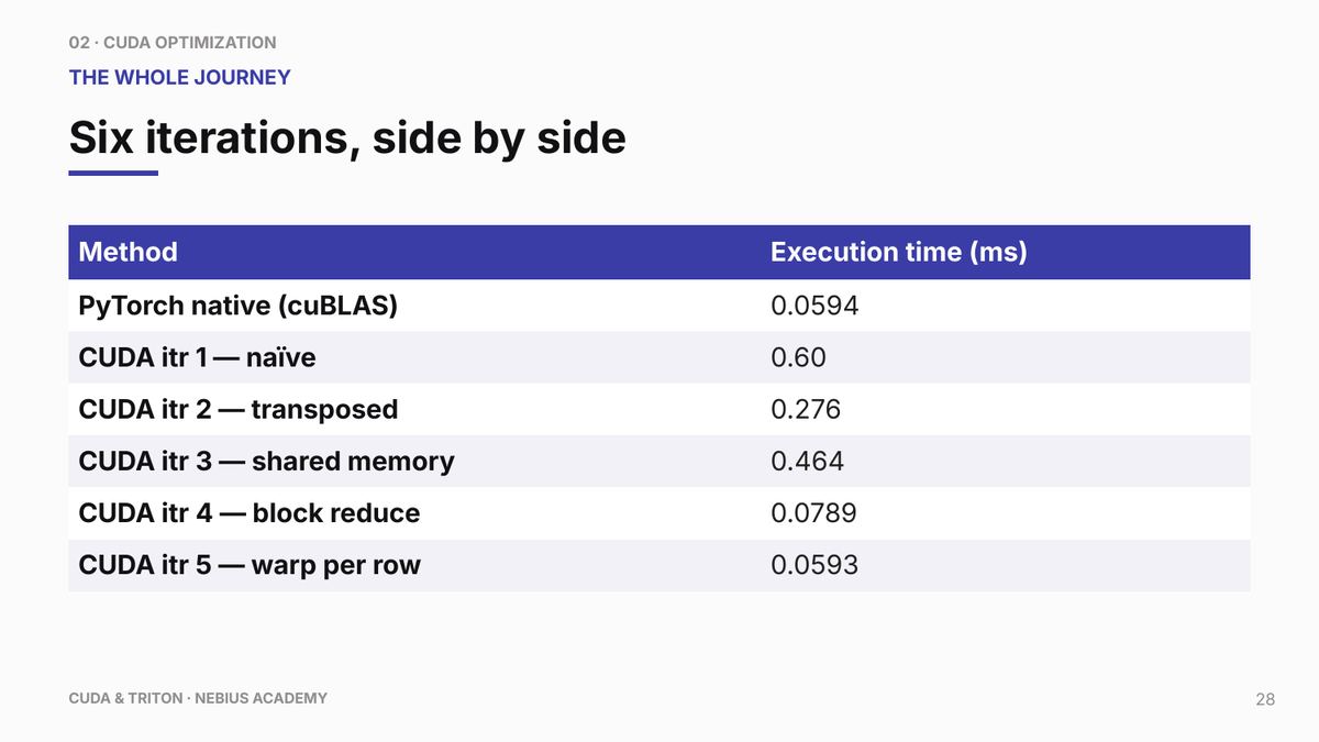
The table records 0.0594 ms for PyTorch/cuBLAS and 0.60, 0.276, 0.464, 0.0789, and 0.0593 ms for iterations 1 through 5. These are observations from one experiment. The supplied table does not give the original matrix shape, dtype, GPU, software versions, warmup, timing boundary, or correctness tolerance. Those missing settings prevent reproduction or a portable performance ranking. No uncertainty estimate is supplied, so 0.0593 versus 0.0594 ms does not establish a reliable advantage over cuBLAS.

Chart note

Measured or compared: Execution time for six matrix-vector implementations: PyTorch native cuBLAS and CUDA iterations 1 through 5.

Axes, units, and series: No x/y axes are drawn because the source visual is a table. Rows are implementation methods. The single numeric series is execution time in milliseconds.

Interpretation: The reported times do not improve at every iteration: iteration 3 is slower than iteration 2, and iteration 5 is numerically close to the library timing. The table does not identify which hardware effects caused those differences.

Source status: The values are reported course measurements, reproduced as recorded rather than re-measured.

The iteration labels suggest different ways to read a row and combine partial sums. The mechanisms below explain those designs. The timing table alone does not verify the implementation details or their costs. A fresh comparison would need the same shape, dtype, GPU, warmup, timing boundary, and correctness tolerance for every implementation.

• Iteration 1 (Naive): A one-thread-per-output design loops over the columns of each row of A. With row-major storage, adjacent threads reading the same column in different rows use addresses separated by the row width, which can require more memory transactions. The exact cost depends on layout and shape.
• Iteration 2 (Source comparison point): The source records a second iteration, but does not document its layout or thread indexing well enough to attribute a coalescing effect. Use its timing only as a comparison point, not as a mechanism example.
• Iteration 3 (Shared Memory Block Reduce): This design divides columns among threads and combines their partial sums through shared memory and block synchronization (__syncthreads()). Its reported 0.464 ms exceeds iteration 2’s 0.276 ms. Bank conflicts, barrier waits, extra address arithmetic, and reduced occupancy are hypotheses to test, not causes established by these timings.
• Iteration 4 (Cooperating Threads): A row is divided across many threads and reduced at block scope. The useful thread count depends on row width, dtype, occupancy, and synchronization cost.
• Iteration 5 (Warp per Row / Warp-Shuffle): One warp can cooperate on a row and reduce partial sums with register shuffles, avoiding block-wide barriers for that reduction. Whether it approaches cuBLAS depends on the measured shape, dtype, GPU, and timing method.

Distinguishing those hypotheses requires the original kernels and measurements: shared-memory conflict counters, barrier-stall evidence, instruction counts, and register/shared-memory limits would test different possible causes. Those records are not supplied with the table. The following calculation instead shows why a cooperative reduction can preserve the GEMV result. It is an arithmetic trace, not a reconstruction or benchmark of iteration 5.

Worked example: Combining a row across warp lanes

Take one matrix row [1,2,3,4] and vector [2,3,4,5]. Their dot product is \(1\times2+2\times3+3\times4+4\times5=40\). Assign the four products to lanes 0 through 3 of one 32-lane warp. Their register partial sums are [2,6,12,20]. Lanes 4 through 31 hold zero and remain active. For a longer row, lane \(l\) first sums products at columns \(l,l+32,l+64,\ldots\) that are within the row.

A shuffle transfers a register value from one participating lane to another. Consider stages with delta equal to 16, 8, 4, 2, then 1. At every stage all 32 lanes execute other = __shfl_down_sync(0xffffffff, partial, delta). Only lanes with lane + delta < 32 then add other to their partial sum. Each exchange reads the values from before that stage’s additions.

The first three stages add only zeros to lanes 0 through 3, so their values remain [2,6,12,20]. At delta=2, lane 0 reads lane 2’s 12 and becomes 14. Lane 1 reads lane 3’s 20 and becomes 26. At delta=1, lane 0 reads lane 1’s 26 and becomes 40. Only lane 0 writes this row’s output, y[row]=40. The other lanes’ final registers are not separate output elements.

The full mask is valid here because all 32 lanes participate in every exchange with the same mask. Lanes holding zero must not exit early. Reading an inactive source lane is not valid, and a shuffle does not order shared-memory accesses.⁵ A shared-memory alternative writes every lane’s partial sum to a distinct shared slot, lets the whole block reach __syncthreads(), then has one thread read and add the slots. A parallel shared-memory tree also needs ordering between stages. These methods combine the same products but use different storage and synchronization. Neither has a universal timing advantage, and floating-point addition order can change rounding.

Launch overhead often becomes visible in small-batch decode because each kernel does little work. A CUDA launch has a nonzero host-side cost whose size depends on the software stack, hardware, synchronization, and measurement method. For sufficiently small operations, that fixed cost can exceed device execution time. The knee on a size-versus-latency plot is the measured transition for one operation and environment. Below it, launch cost dominates, while larger inputs eventually expose memory or compute limits.

3.8 CUDA launch and indexing example

This CUDA-like pseudocode connects one-dimensional tensor indexing to a launch configuration. It shows block and thread indices, a grid-stride loop, and the access pattern needed for coalescing. Allocation, data transfer, synchronization, and cleanup are outside this example.

Worked example: Grid-stride vector add

Assume contiguous inputs x=[0,1,2,3,4,5,6,7,8,9] and y=[10,10,10,10,10,10,10,10,10,10], with space for ten output elements. The example deliberately launches grid=2, block_size=4, so eight logical threads cover n=10 elements with stride \(2\times4=8\).

Block 0, thread 0 starts at index 0 and writes out[0]=0+10=10. Its second loop iteration visits index \(0+8=8\) and writes out[8]=8+10=18. Its next candidate, 16, is outside the input, so the loop stops. Block 0, thread 1 visits indices 1 and 9 and writes 11 and 19. Global thread IDs 2 through 7 each visit their first index only, writing 12 through 17, because their next indices are at least 10. The complete result is [10,11,12,13,14,15,16,17,18,19], with every element written once.

The alternative full-coverage launch, grid=ceil(n/block_size)=3, exposes twelve threads and stride 12. It gives each valid thread one element, while IDs 10 and 11 do no work. In both launches, the stride counts all logically launched threads, not just those simultaneously resident on SMs. Hardware may schedule the blocks at different times without changing this coverage.

Code example: Grid-stride vector add

kernel vector_add(x, y, out, n):
    tid = blockIdx.x * blockDim.x + threadIdx.x
    stride = blockDim.x * gridDim.x
    for i in range(tid, n, stride):
        out[i] = x[i] + y[i]

n = 10
block_size = 4
launch grid = 2, block = block_size
# Alternative full coverage: grid = ceil(n / block_size)

Conclusion: Thread mapping, address order, and grid-stride coverage shape coalescing and work balance. For transfer, synchronization, and cleanup costs, see the copy examples in Section 3.3.1 and the ordering rules in Section 3.4. Triton keeps the mapping concerns but expresses them through program instances, tiles, offsets, masks, and compiler-selected lower-level execution.

---

1. NVIDIA. (2024). CUDA C++ Programming Guide 12.4. https://docs.nvidia.com/cuda/archive/12.4.0/cuda-c-programming-guide/index.html (release 2024-03-05). Support: streams, events, page-locked host memory, peer access, coalesced device access, and L2 persistence controls used in Sections 3.3, 3.4, and 3.6. Limit: overlap also requires pinned memory, independent work, and hardware support, as stated in the chapter.

2. NVIDIA. (2024). CUDA C++ Programming Guide 12.4. https://docs.nvidia.com/cuda/archive/12.4.0/cuda-c-programming-guide/index.html (release 2024-03-05). Support: streams, events, page-locked host memory, peer access, coalesced device access, and L2 persistence controls used in Sections 3.3, 3.4, and 3.6. Limit: overlap also requires pinned memory, independent work, and hardware support, as stated in the chapter.

3. NVIDIA. (n.d.). cuBLAS Library (versioned cuBLAS 13.4 documentation). https://docs.nvidia.com/cuda/cublas/. Support: cuBLAS as the CUDA BLAS implementation with GEMM, GEMV, and batched variants behind the library API. Limit: the guide’s dispatch and baseline recommendation is course guidance; exact kernel selection depends on shape, dtype, and version.

4. NVIDIA. (2023). Matrix Multiplication Background User’s Guide (last updated 2023-02-01). https://docs.nvidia.com/deeplearning/performance/dl-performance-matrix-multiplication/index.html. Support: GEMM tiling approach and the statement that matrix-vector products with M = 1 or N = 1 are always memory limited. Limit: arithmetic intensity comparison is a rule of thumb that omits instruction overhead and on-chip hierarchy effects.

5. NVIDIA. (2024). CUDA C++ Programming Guide 12.4. https://docs.nvidia.com/cuda/archive/12.4.0/cuda-c-programming-guide/index.html (release 2024-03-05). Support: streams, events, page-locked host memory, peer access, coalesced device access, and L2 persistence controls used in Sections 3.3, 3.4, and 3.6. Limit: overlap also requires pinned memory, independent work, and hardware support, as stated in the chapter.