1  LLM Workloads and Performance Limits

Connect workload phases, live tensor state, resource limits, measurements, and software controls so performance work begins with a measurable bottleneck and its responsible layer.

Training and serving run related model operations, but they keep different tensors (multidimensional arrays of numbers) in memory and move different bytes during each phase. Explaining their performance starts with the different results they produce.

During training, the model receives examples and predicts outputs. A loss (a single number measuring how wrong the predictions are) compares those predictions with target answers, backward propagation computes how the loss depends on the weights (the model’s learned numbers, also called parameters), and an optimizer (the update rule) changes those weights. During text generation, the weights stay fixed: the model processes a prompt, produces scores for the next token (a word or word fragment that the model reads and writes as one unit), and a selection rule chooses that token. Repeating this step extends the output. The initial prompt processing is called prefill, and the repeated one-token steps are decode. Retained attention state (Section 1.1), called the key-value (KV) cache, lets later steps reuse earlier work. Evaluation also keeps weights fixed, but compares predictions with reference answers to measure quality.

To explain a measured slowdown, first identify the phase, such as training backward or one-token decode. Then list the tensors and buffers that remain live, estimate which bytes move, and measure the compute, memory, launch, communication, and waiting behavior in that phase. These steps narrow the problem to the limiting resource or wait and to the controls that can change it.

A bottleneck is the resource or dependency that currently limits one measured execution region. It is not a permanent label for the whole model: a training forward pass, an optimizer update, prompt prefill, one-token decode, and distributed synchronization can each be limited by a different resource.

The figure below follows both workloads through the same model parameters.

Figure 1.1: Training and inference serving use shared parameters but keep different state live.

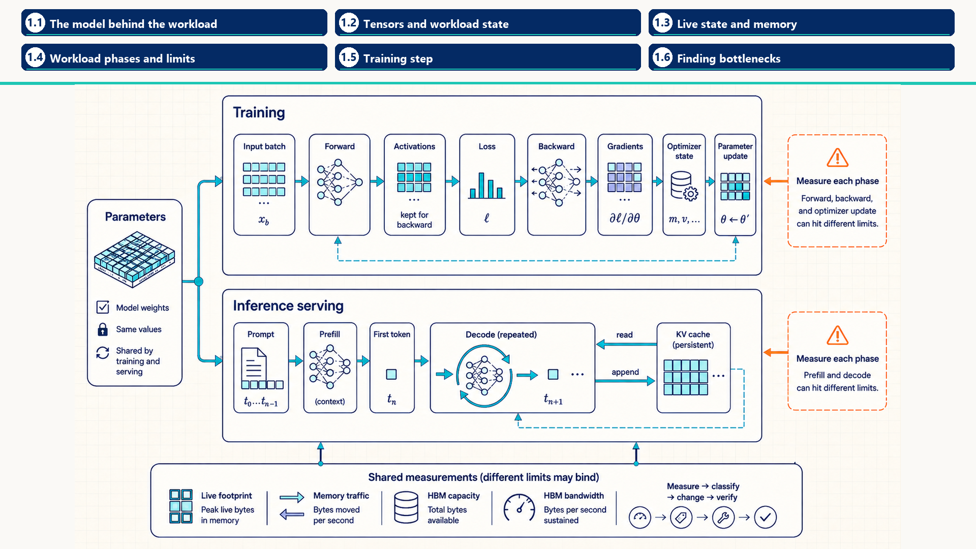
The upper path follows activations, loss, gradients, optimizer state, and parameter update during training (the training objects defined in Section 1.3). The lower path separates prompt prefill from repeated decode and shows the KV cache as persistent state that decode reads and appends. A profiler (a tool that records where time and memory go) or a memory-statistics pass can measure capacity, traffic, and bandwidth for the active phase rather than assigning them to the whole model.

1.1 The model behind the workload

Every measurement in this guide observes part of one computation: turning a sequence of tokens into scores for the next token. Questions such as “why is decode slow?” or “why does training run out of memory?” are answered by locating the part of that computation that is slow or large. That requires a picture of its parts and their sizes before any hardware enters the discussion.

Text first becomes numbers. A tokenizer (software that splits text into tokens and maps each one to an integer) produces token IDs (positions in a fixed list of tokens, the vocabulary). Llama 3 uses a vocabulary of about 128,000 tokens.¹ Section 8.1 treats tokenizers and why the token count drives cost. From there, a Llama-style decoder-only language model applies four stages; other model families can use different normalization and feed-forward choices:

1. Embedding: Each token ID selects one row of an embedding table (a matrix holding one learned vector per vocabulary entry). The vector has \(d\) numbers, the hidden width or model dimension. A sequence of \(T\) tokens therefore becomes a \(T\times d\) matrix, the hidden state.
2. Layers: The hidden state passes through \(L\) structurally similar layers, also called transformer blocks, with separately learned weights. Each layer has two sub-layers, and each sub-layer follows the same pattern: normalize its input, transform it, and add the result back to the input.
   • The attention sub-layer first applies RMSNorm (it rescales each token’s vector to a standard size). Three projections (multiplications by learned weight matrices) then produce a query, a key, and a value vector for every token. Attention (the operation that lets each token combine information from other tokens) compares each token’s query with the keys of the permitted positions and mixes the matching values. In a causal language model, a token may use only itself and earlier positions. Attention is split into several attention heads (independent attention calculations on slices of the hidden width), each with vectors of length \(d_h\), the head dimension. An output projection maps the result back to width \(d\). Section 4.7 works through the attention arithmetic.
   • The feed-forward sub-layer applies another RMSNorm and then a multilayer perceptron (MLP) (a pair of large projections with a nonlinear function between them) to each token independently. Llama-style models use the SwiGLU form, which has three weight matrices and widens each token’s vector from \(d\) to an intermediate width \(d_{ff}\) and back.²
   • A residual connection (adding a sub-layer’s output to its input) follows each sub-layer, so the hidden state keeps its \(T\times d\) shape from layer to layer.
3. Output: A final RMSNorm and the language-model head (a \(d\times V\) projection, where \(V\) is the vocabulary size) turn the hidden state into logits: one unnormalized score per vocabulary entry for each position.
4. Selection: A decoding rule turns the last position’s logits into the next token, as described at the end of this section.

Almost all parameters sit in the projection matrices of stage 2, and every projection multiplies the \(T\times d\) hidden state by a weight matrix. This matrix multiplication is the operation that GPU hardware (Chapter 2) and GPU libraries (Chapter 3) are built to accelerate. Attention itself has no weights, but its work and its stored state grow with the number of tokens, which is why the KV cache receives separate treatment in Section 1.3 and Chapters 8 and 9.

Worked example: Where the parameters of an 8B model sit

Inputs: The published Llama 3 8B configuration has \(L=32\) layers, \(d=4{,}096\), 32 query heads and 8 key-value heads with \(d_h=128\), an MLP width \(d_{ff}=14{,}336\), and a vocabulary of about 128,000 tokens.³ Sharing each key and value head among four query heads is called grouped-query attention (Section 1.3), so the key and value projections produce \(8\times128=1{,}024\) numbers per token instead of 4,096.

Table 1.1: Parameters in one layer of the Llama 3 8B configuration.

Weight matrix in one layer	Shape	Parameters
Query projection	\(4{,}096\times4{,}096\)	16,777,216
Key projection	\(4{,}096\times1{,}024\)	4,194,304
Value projection	\(4{,}096\times1{,}024\)	4,194,304
Attention output projection	\(4{,}096\times4{,}096\)	16,777,216
MLP gate and up projections (two matrices)	\(4{,}096\times14{,}336\) each	117,440,512
MLP down projection	\(14{,}336\times4{,}096\)	58,720,256
Two RMSNorm weight vectors	\(4{,}096\) each	8,192
Layer total		218,112,000

Whole model: The 32 layers hold \(32\times218{,}112{,}000=6{,}979{,}584{,}000\) parameters. The embedding table and the language-model head each hold about \(128{,}000\times4{,}096=524{,}288{,}000\) when they are separate matrices. The total is about 8.03 billion, consistent with the model’s name. A tied design reuses the embedding matrix for the output projection and would reduce this illustrative total by about 0.52 billion parameters.

Conclusion: About 81 percent of each layer’s parameters sit in the MLP, and nearly all the rest in the four attention projections. Every generated token passes through all of these matrices, so their size in bytes sets how much data each decode step must read, whether it advances one request or a whole batch (Section 2.8).

The final stage chooses one token from the logits. Softmax (exponentiating each score and dividing by the sum, so the scores become probabilities, Section 4.7) converts logits into a probability distribution over the vocabulary. A decoding rule then selects from it:⁴

• Greedy decoding picks the most probable token. It is deterministic in principle: the same prompt and the same arithmetic give the same output, although changes in batching or kernel choice can alter floating-point rounding enough to flip a close choice.
• Temperature uses \(t>0\) to divide the logits before softmax. Values between 0 and 1 concentrate probability on likely tokens, and values above 1 spread it out. A setting of zero, when an API supports it, selects a special decoding rule rather than evaluating division by zero.
• Top-k sampling draws randomly from only the \(k\) most probable tokens.
• Top-p (nucleus) sampling orders tokens from highest to lowest probability, keeps the shortest prefix whose probabilities add up to at least \(p\) for \(0<p\leq1\), and samples after renormalizing that prefix.
• Beam search keeps several candidate continuations at once and extends the most probable ones, so it runs several sequences per request.

Selection runs once per generated token for every request. Its arithmetic is small next to the layers, but it can require sorting a vocabulary-sized vector or a round trip to the CPU, and random selection makes repeated runs differ. Chapter 10 returns to its serving cost, and Chapter 11 to its effect on correctness checks. The next section turns from the model’s mathematical parts to the stored arrays that a measurement actually records.

1.2 Tensors and workload state

Section 1.1 named the model’s parts in mathematical terms. A performance measurement records the same parts as stored arrays: how many bytes each occupies, where it lives, and how its elements are laid out. Parameters, activations, gradients, logits, loss, and KV cache each carry a distinct storage and lifetime cost.

A tensor has a mathematical meaning and a physical storage description at the same time. Mathematically, it is a scalar, vector, matrix, or higher-dimensional array used in the model computation. Physically, it is a descriptor over storage: shape, dtype, strides, device, layout, storage offset, and sometimes gradient metadata. Performance depends on both descriptions. The PyTorch 2.4 documentation in Tensor Attributes describes dtype, device, layout, strided storage, and stride semantics used in this chapter.⁵

• Mathematical tensor: The array used in an operation, such as a vector of token embeddings, a matrix of weights, or a batch of logits.
• Tensor storage: The underlying bytes allocated on CPU memory, GPU High Bandwidth Memory (HBM) (the GPU’s large main memory, Section 2.3), pinned host memory (CPU memory locked in place so the GPU can copy it directly, Section 2.6), or another device-visible memory tier.
• Shape: The logical dimensions of the tensor. Shape controls matrix sizes, attention dimensions, batch sizes, and whether operations can use efficient kernels (functions that run on the GPU, Section 2.2).
• Dtype: The numeric representation, such as FP32, BF16, FP16, FP8, INT8, or INT4 (32-bit, 16-bit, 8-bit, and 4-bit floating-point and integer formats, Section 7.4). Dtype controls bytes per element and can change which kernels are legal or fast.
• Device: Where the tensor lives, such as CPU memory or cuda:0. Device placement controls which implementation PyTorch dispatches (selects and calls) and determines whether hidden transfers are needed.
• Strides and layout: The mapping from logical indices to storage offsets. Strides determine whether nearby logical elements are nearby in memory and whether a tensor is contiguous.
• Autograd metadata: Training-time metadata used by PyTorch autograd (its automatic-differentiation engine) to know which operations produced a tensor and how to compute gradients.
• Loss: A scalar or reduced tensor that measures how far the model output is from the training target and supplies the starting value for backward propagation.

This distinction explains several later performance issues. A transpose can be mathematically cheap while creating a non-contiguous view. A dtype change can halve memory traffic while selecting a different kernel path. A tensor’s device determines whether a copy is required. Autograd metadata can extend a tensor’s lifetime through backward propagation.

The next section names the persistent and temporary model objects that use this storage. Their lifetimes, rather than their mathematical names alone, determine peak memory and data movement.

Worked example: Inspecting tensor identity

This example requires PyTorch and an available CUDA device (an NVIDIA GPU usable through CUDA, NVIDIA’s GPU programming platform, Chapter 3). For the contiguous 2 x 3 FP16 tensor below, expect shape (2, 3), dtype torch.float16, device cuda:0 or another selected CUDA device, stride (3, 1), True for contiguity, and 12 bytes of tensor payload. The device label can vary with the selected GPU.

Code example: Inspecting tensor identity

import torch

x = torch.randn(2, 3, device="cuda", dtype=torch.float16)

print(x.shape)
print(x.dtype)
print(x.device)
print(x.stride())
print(x.is_contiguous())
print(x.numel() * x.element_size(), "bytes")

Conclusion: The trace separates the logical 2 x 3 FP16 array from its physical storage. Its six values occupy 12 bytes, while its stride and device determine later kernel and transfer consequences.

Worked example: Counting parameter and gradient bytes

This abbreviated calculation assumes that model already exists. Parameter bytes can be counted immediately. Gradient bytes appear only after backward propagation has populated p.grad. The result covers tensor payloads, not allocator reservation, fragmentation (free memory split into pieces too small to use), metadata, workspaces, or distributed buffers.

Code example: Counting parameter and gradient bytes

import torch

param_bytes = sum(
    p.numel() * p.element_size()
    for p in model.parameters()
)

grad_bytes = sum(
    p.grad.numel() * p.grad.element_size()
    for p in model.parameters()
    if p.grad is not None
)

print(f"parameters: {param_bytes / 2**20:.1f} MiB")
print(f"gradients:  {grad_bytes / 2**20:.1f} MiB")

Conclusion: Parameter payload exists before backward, while gradient payload begins when autograd materializes p.grad. A memory report therefore needs the active phase as well as allocator and workspace overhead.

The same tensor properties appear in two distinct execution regimes. Training changes parameters and retains backward state. Inference serving keeps parameters fixed while maintaining request and cache state. The comparison below names the goal, live objects, phases, and measurements for each regime.

• Training: Repeated execution that updates model parameters from data.
  • Goal: Improve the objective while maximizing useful tokens per second, numerical stability, and hardware utilization.
  • Live objects: Parameters, activations, gradients, optimizer state, temporary workspaces, and often communication buffers (all defined in the next section).
  • Phases: Forward propagation, loss computation, backward propagation, optimizer step, and distributed synchronization when multiple ranks (cooperating processes, usually one per GPU, Section 2.5) are used.
  • Measurements: Training tokens per second, step time, time to target quality, memory headroom, scaling efficiency, and numerical stability.
• Inference serving: Request-driven execution that generates outputs with fixed model parameters.
  • Goal: Meet latency, throughput, quality, and cost targets under a service workload.
  • Live objects: Parameters, temporary activations, KV cache, scheduler metadata, request queues, sampling state (the selection rule’s settings and random state), and sometimes communication buffers.
  • Phases: Tokenization, request admission, prefill, decode, post-processing, and streaming.
  • Measurements: Serving measurements describe waiting, streaming speed, and completed work. Chapter 8 develops these quantities and their measurement boundaries.
    • Time To First Token (TTFT): elapsed time from request arrival to the first emitted token.
    • Inter-Token Latency (ITL): the gap between two consecutive emitted tokens.
    • Time Per Output Token (TPOT): for one request with \(n>1\) output tokens, the mean of its \(n-1\) ITL gaps. It excludes first-token latency.
    • End-to-end latency: elapsed time from arrival to completion.
    • Throughput: completed requests or tokens per second for the stated workload.
    • Goodput: completed work per second that meets the specified service targets, such as latency and quality limits in a Service-Level Objective (SLO, Section 8.3).

Training and inference now have concrete meanings: each mode is a sequence of phases operating on named state objects. The next section follows the objects that remain live as those phases execute.

1.3 Live state and memory

Section 1.2 defined the individual objects. Memory pressure depends on which of those objects overlap in time. Parameters and optimizer buffers may stay live for the whole training step. Saved activations accumulate during forward. Gradients appear during backward. Temporary workspaces can raise the peak even though they exist briefly. In serving, model weights remain fixed while admitted requests grow and release KV-cache blocks.

• Parameters: Learned weights. They are used in both training and inference. Footprint scales with parameter count and dtype. For example, a 7B-parameter model in FP16 or BF16 is roughly 14 GB before metadata, fragmentation, and engine overhead.
• Activations: Intermediate tensors produced by forward propagation. Training often saves them for backward propagation. Inference usually releases most of them quickly. Footprint scales with batch size, sequence length, hidden dimension, layer count, precision, and checkpointing policy.
• Gradients: Derivatives of the loss with respect to parameters. They are training state. Their footprint is often parameter-sized before sharding, accumulation strategy, or reduced-precision storage changes it.
• Optimizer state: Extra buffers used by optimizers such as Adam or AdamW (update rules that keep running averages of each gradient and its square). Adam-style first and second moments can exceed the parameter footprint when stored in FP32, which is why optimizer state becomes a training memory wall. Adam maintains biased first and second moment estimates as described in Adam: A Method for Stochastic Optimization⁶, and ZeRO partitions optimizer states, gradients, and parameters across data-parallel ranks as described in ZeRO: Memory Optimizations Toward Training Trillion Parameter Models⁷.
• Temporary workspaces: Short-lived buffers allocated by kernels, vendor libraries, compilers, or serving engines. They affect peak memory and can cause out-of-memory failures.
• Key-value (KV) cache: Inference-serving attention state that stores previous keys and values so decode does not recompute the full prefix.
• Communication buffers: Intermediate tensors used for collective operations (communication steps in which every participating rank takes part), such as all-reduce (every rank ends with the sum of all ranks’ tensors), all-gather, reduce-scatter, and all-to-all (Section 12.6), or for point-to-point transfers. They appear in distributed training and distributed inference and can create memory spikes as well as network traffic.
• Request and scheduler metadata: Serving-engine state that tracks request IDs, token positions, sampling constraints, KV block tables (Section 9.5), prefix-cache entries (Section 10.5), queue state, and admission decisions. It is smaller than tensor state but can affect launch gaps, queueing, and cache correctness.

A model that fits in one mode may fail in another. A model checkpoint (the saved weights file) that fits for inference may not fit for training once gradients and optimizer state are added. A model that fits short prompts may fail under long-context serving because KV cache grows with admitted requests and sequence length.

Worked example: Training memory per parameter

Inputs: Consider the mixed-precision training arrangement (computing mostly in 16-bit formats while keeping some values in 32-bit) used for the ZeRO paper’s Adam memory estimate. It keeps five values for every parameter. The working weights and gradients in the cited example use FP16, at 2 bytes each. Using BF16 for these two arrays gives the same byte count. The optimizer holds an FP32 master copy of the weights plus Adam’s two running averages, at 4 bytes each. Section 7.4 explains why the master copy exists. Other implementations can store gradients or optimizer state differently, so this 16-byte budget applies to the arrangement specified here.

Calculation: \(2+2+4+4+4=16\) bytes per parameter. This is the standard accounting in the ZeRO paper, which writes the optimizer’s share as \(K=12\) bytes.⁸ For a 7-billion-parameter model, \(7\times10^9\times16=112\times10^9\) bytes, or 112 GB, compared with 14 GB for the BF16 weights that inference needs.

Conclusion: Before a single activation is stored, the training state of a 7B model exceeds one 80 GB GPU. Activation checkpointing (discarding some forward results and recomputing them during backward, Section 7.2) does not help with these 112 GB, because it reduces activations only. Sharding the 16 bytes across ranks (Section 13.4) does.

Peak-memory lifecycle

Before forward: Parameters, input tensors, and persistent buffers are live. Optimizer state is also live after initialization, although some optimizers allocate their buffers lazily at the first update. The model may appear to fit at this point while the upcoming step still cannot run.

During forward: Each layer produces activations. Training keeps many of them alive because backward propagation uses the original values. Inference usually releases most temporary activations quickly.

At loss and backward start: The loss is the starting point for backward traversal of the autograd graph. Backward reads saved activations, writes gradients, and may allocate temporary workspaces for backward kernels.

During optimizer step: Adam-style optimizers read parameters, gradients, first moments, and second moments, then write updated state. This phase can be limited by memory bandwidth even if the forward pass was limited by matrix arithmetic.

After step: Gradients may be set to None and activations are released, but allocator-reserved memory can remain high because the PyTorch caching allocator (which keeps freed GPU memory blocks for reuse instead of returning them, Section 3.3.2) keeps blocks for reuse.

The cache stores the key and value vectors that attention compares against (Section 1.1). Later tokens’ queries are compared with these stored keys to determine attention weights, which combine the corresponding values. A KV head supplies one key vector and one value vector per token position in a layer. Several query heads can share that pair, as in grouped-query attention (GQA), so the cache counts KV heads rather than automatically counting query heads.⁹ Here each key and value has \(d_h\) scalar components, where \(d_h\) is vector width, not the number of heads or the model’s full hidden width. Section 4.7 works through the attention calculation.

In a transformer with the same attention layout in every layer, cache entries therefore have four identifying indices: retained token position, layer, KV head, and vector component, with separate key and value arrays. Without cross-request prefix sharing, a first payload estimate is

\[ M_{\mathrm{KV}}=2N_{\mathrm{tok}}LH_{\mathrm{kv}}d_hb. \tag{1.1}\]

Here \(N_{\mathrm{tok}}\) is the total number of retained token positions across admitted requests, which is \(B\times T\) for \(B\) sequences of \(T\) tokens each. \(L\) is the layer count, \(H_{\mathrm{kv}}\) the KV-head count, \(d_h\) the head dimension, and \(b\) the bytes per cache element. Chapter 8 uses the same symbols. Allocator blocks and engine metadata add overhead. Mixed attention layouts require a layer-by-layer sum instead. Chapter 8 applies this estimate to concurrency and capacity, while Chapter 9 explains how the cache is laid out and accessed.

Worked example: From one cached token to 256 MiB

For one retained token in one layer and one KV head, the key and value contain \(2\times128=256\) scalars. Eight KV heads require \(256\times8=2{,}048\) scalars per layer. Across 32 layers this becomes \(2{,}048\times32=65{,}536\) scalars for that token, or \(65{,}536\times2=131{,}072\) bytes in BF16. Keeping 2,048 token positions requires \(131{,}072\times2{,}048=268{,}435{,}456\) bytes, or 256 MiB. These are the factors \(d_h=128\), \(H_{\mathrm{kv}}=8\), \(L=32\), \(b=2\), and \(N_{\mathrm{tok}}=2{,}048\) in the formula. This is the raw cache payload. Allocator blocks, metadata, and other live state still require headroom.

1.4 Workload phases and limits

Diagnosing a phase requires fixed meanings for the words used to describe speed, because “fast” can refer to one request, a whole service, or one piece of hardware. The rest of the guide uses these meanings:

• Latency: elapsed time for one piece of work, from its start to its completion, such as one training step or one request.
• Throughput: completed work per unit of time across many pieces of work, such as tokens per second or requests per second. Processing work in larger batches often raises throughput while raising each item’s latency.
• Bandwidth: the rate at which a memory or link can move bytes. An H100 SXM GPU’s HBM is specified at 3.35 TB/s (Section 2.7). Achieved bandwidth is the measured bytes divided by the measured time.
• Utilization: the fraction of a resource’s capacity, or of the time, that is in use. A utilization figure is meaningful only with its resource and definition. The “GPU utilization” reported by monitoring tools is a narrow time measure (Section 5.1).
• Saturation: a resource running at its limit, so that additional demand waits in a queue instead of being served faster.
• Critical path: the longest chain of dependent work in a step. Only shortening work on this chain shortens the step, and work that overlaps it is hidden.
• Steady state: repeated execution after one-time setup, such as compilation, memory allocation, and cache filling, has finished. Measurements in this guide refer to steady state unless they say otherwise.

Check footprint by asking whether the live objects fit. Check traffic by asking how many bytes the phase reads and writes. Check throughput by asking how quickly the hardware can perform those transfers or calculations. Diagnose a phase by measuring these separately. Fitting in HBM does not show that HBM bandwidth is sufficient.

• Bandwidth and locality: The rate and distance at which bytes must reach the computation. Reuse in on-chip storage (registers, shared memory, or cache, Section 2.3) reduces traffic to slower memory tiers.
• Compute throughput: The rate of useful arithmetic work for the phase, interpreted together with tensor shapes, precision, and hardware utilization.
• Launch and control overhead: Time spent in Python dispatch, framework dispatch, kernel launches, compiler transitions, or scheduler decisions.
• Communication and synchronization: Time spent moving tensors across GPUs or ranks and waiting for participants to reach compatible execution points.

Diagnose one phase at a time by naming the work, the live objects, the target measurement, and the resource whose capacity, throughput, or dependency is exhausted.

• Training forward: Reads parameters and input batches, writes activations, and often uses large matrix operations that run on Tensor Cores (the GPU’s dedicated matrix-multiply units, Section 2.4). Likely bottlenecks are compute throughput, activation memory, and HBM traffic. Developed in Chapters 2 through 5 and revisited in Chapters 7 and 13.
• Training backward: Reads saved activations and parameters, writes gradients, and may recompute activations when activation checkpointing is used. Likely bottlenecks are activation memory, HBM bandwidth, and gradient computation. Developed in Chapters 5, 11, and 13.
• Optimizer step: Reads parameters, gradients, and optimizer state, then writes updated parameters and state. Likely bottlenecks are memory bandwidth and optimizer-state footprint. Developed in Chapters 1, 7, and 13.
• Prefill: Processes prompt tokens and builds initial KV cache. It often forms large matrix operations over many tokens and can be compute-heavy. Likely bottlenecks are compute throughput, temporary activation and workspace memory, and attention traffic for long prompts. Developed in the inference, serving, and implementation chapters (8, 10, and 11).
• Decode: Generates one token at a time while reading parameters and the existing KV cache, then appending new KV entries. Likely bottlenecks are HBM bandwidth, launch overhead, batching, and cache layout. Developed in Chapters 6, 8, 9, and 10.
• Distributed synchronization: Moves gradients, parameters, activations, routed tokens for mixture-of-experts layers (Section 13.5), or partial layer results between ranks. Likely bottlenecks are interconnect bandwidth, latency, topology, rank skew (ranks reaching a shared step at different times), and collective scheduling. Developed in Chapters 12 and 13.

A first estimate of dense projection arithmetic uses the number \(N_p\) of weights participating in those projections. Each such weight contributes one multiplication and one addition per token, giving about \(2N_p\) floating-point operations (FLOPs) (individual arithmetic operations, counted precisely in Chapter 5) per token. Backward propagation costs about twice the forward pass, so training costs about \(6N_p\) FLOPs per token.¹⁰ This estimate omits embedding lookup, normalization, and other smaller operations; an embedding lookup does not multiply every entry in its table. The cited scaling-law estimate excludes embedding parameters. Attention adds a term that grows with context length. That term is small when the context is short relative to the hidden width.

Worked example: Arithmetic per token for an 8B model

Inputs: Use \(N_p=8\times10^9\) as a rough proxy for the dense projection parameter count at the Llama 3 8B scale from Section 1.1, with the attention term ignored. This rounded estimate is not an exact operation count for that model’s embedding and output layers.

Inference: One forward pass per generated token costs \(2\times8\times10^9=1.6\times10^{10}\) FLOPs, or 16 GFLOP.

Training: One training token costs \(6\times8\times10^9=4.8\times10^{10}\) FLOPs. Training on \(10^{12}\) tokens therefore costs \(4.8\times10^{22}\) FLOPs. One H100 SXM running at its dense BF16 peak of about \(989\) TFLOP/s (Section 2.8) would need \(4.8\times10^{22}/9.89\times10^{14}\approx4.9\times10^{7}\) seconds, about 560 days, and real runs achieve only a fraction of peak.

Conclusion: Training cost scales with parameters times tokens, which is why training uses many GPUs (Chapter 13). A generated token needs only 16 GFLOP, about 16 microseconds at peak rate. Reading the model’s 16 GB of BF16 weights at 3.35 TB/s takes about 4.8 milliseconds, roughly 300 times longer. Section 2.8 explains why that data movement, not the arithmetic, sets the time of a small decode step.

Moving bottlenecks are normal. Removing recomputation can expose memory bandwidth. Increasing batch size can expose KV-cache capacity. Sharding model state can expose network synchronization. The engineering task is to follow the bottleneck as each change exposes a new constraint.

1.5 Training step

Section 1.4 identified the measurements and resource limits that can change across workload phases. A supervised training loop makes those phases concrete. Each repeated step moves input data to the GPU, runs forward computation to produce predictions, compares predictions with labels through the loss function, computes gradients through backward propagation, updates parameters through the optimizer, and may synchronize distributed workers. Later chapters improve these same moments through placement, kernels, precision, graph capture (recording a sequence of operations so it can be optimized or replayed, Chapter 6), sharding, and communication scheduling.

• Forward propagation: Reads inputs and parameters, writes outputs, and may save activations for backward propagation.
• Loss computation: Turns predictions and labels into the scalar or batched objective being optimized.
• Backward propagation: Traverses the recorded computation in reverse to produce gradients.
• Optimizer step: Updates parameters using gradients and optimizer state.
• Device placement: Determines whether tensors live on CPU memory, GPU HBM, or another device, and therefore which transfers and execution paths the step uses.

In the code below, each line identifies a live object, a resource it can stress, and a software layer that can own the likely fix.

Worked example: Minimal training loop

This abbreviated workload trace uses sequence classification: each input sequence has one class label. input_ids is a torch.long tensor of shape [B,T], with batch size B and a fixed sequence length T; no padding is used in this example. The supplied classifier returns a floating-point logits tensor [B,C] directly, with C class scores per sequence, not a structured output object or [B,T,C] token scores. labels has shape [B], dtype torch.long, and values from 0 to C-1. The model is in training mode on cuda:0, and optimizer was constructed for those parameters after device placement. loader supplies compatible batches. Constructors are omitted.

nn.CrossEntropyLoss() takes the raw logits and labels and returns a scalar with its default mean reduction. For B=2, C=2, logits [[0,0],[0,0]], and labels [0,1], each row gives the target probability 1/2. Each example’s loss is -log(1/2), about 0.6931, and their mean is also 0.6931. This scalar supplies the starting point for loss.backward(). The class axis and target type follow the PyTorch 2.4 loss contract.¹¹ A causal language model needs a separate token-target alignment and loss layout. This classifier trace does not specify that task.

Code example: Minimal training loop

import torch
import torch.nn as nn

device = torch.device("cuda", 0)
# model is already on this device; optimizer owns its parameters.
loss_fn = nn.CrossEntropyLoss()

for batch in loader:
    # Pinned source buffers plus non_blocking copies can overlap input transfer with GPU work.
    input_ids = batch["input_ids"].to(device, non_blocking=True)
    labels = batch["labels"].to(device, non_blocking=True)

    # Releasing old gradient storage avoids writing a full tensor of zeros each step.
    optimizer.zero_grad(set_to_none=True)

    # Forward execution reads parameters, creates activations, and may retain them for backward.
    logits = model(input_ids)  # tensor [B, C], one row per sequence

    # Integer labels [B]; default mean reduction returns a scalar.
    loss = loss_fn(logits, labels)

    # Backward reads saved activations, writes gradients, and may trigger distributed collectives.
    loss.backward()

    # The optimizer reads and writes parameters, gradients, and optimizer-state buffers.
    optimizer.step()

What the training step makes measurable

Input transfer: The .to(device, non_blocking=True) calls are only asynchronous when the source path and stream dependencies permit it. Pinned host memory is commonly needed for useful overlap, and a stream (an ordered queue of GPU work, Section 3.4) determines what must wait. The CUDA C++ Programming Guide (12.4) documents page-locked host memory and overlap of data transfer with kernel execution.¹²

Forward execution: PyTorch dispatches a graph of tensor operations. Large projections may call vendor GEMM (General Matrix-Matrix Multiplication, Section 3.7) kernels, while small elementwise regions may launch separate kernels unless compilation or fusion (combining several operations into one kernel, Section 4.6) changes the path.

Activation retention: Autograd records operations and saves tensors needed for backward. The overlap of parameters, saved activations, gradients, and workspaces usually places peak training memory before or during backward.

Backward execution: Backward kernels consume saved activations and parameters to produce gradients. In distributed data-parallel training, gradient buckets (groups of gradients sent together) may start all-reduce while earlier layers are still computing backward.

Optimizer state traffic: Adam-style updates often spend most of their time reading and writing parameter, gradient, and moment buffers.

Memory-reduction options: Activation checkpointing trades recomputation for lower saved-activation memory. Fully Sharded Data Parallel (FSDP) and Zero Redundancy Optimizer (ZeRO) shard model state across ranks, so that each rank stores only part of it. Each changes a different object or lifetime, so the profiler must identify which state limits the run.

Distributed additions: Distributed Data Parallel (DDP) adds gradient synchronization to this loop. FSDP also changes where parameters, gradients, and optimizer state live and when they are gathered or scattered. Chapter 13 develops both.

Conclusion: The trace makes input transfer, retained activations, gradients, optimizer state, and distributed state observable as separate parts of one training step. Their measured peak and duration identify which memory or execution change belongs next.

Inference serving introduces a different live-state profile, including KV cache, request scheduling, prefix reuse, and speculative decoding (a cheap model proposes several tokens and the full model checks them at once, Section 10.6). Chapter 8 begins that transition.

1.6 Finding bottlenecks

Finding a bottleneck connects a measured phase and its live state to the software or hardware layer that controls the limiting resource. The result is a targeted change with a measurable end-to-end effect.

1.6.1 Bottleneck classes and optimization levers

A measurement names the slow region. The next decision is what kind of limit that region hits, because each kind has its own family of fixes. Two classifications organize the rest of the guide: bottleneck classes describe what limits a region, and optimization levers describe what a change does.

A region’s bottleneck class names the resource or wait that sets its duration. Each class assignment describes one measured region at one moment, not a permanent label for the whole model:

Table 1.2: Bottleneck classes, what sets their duration, and typical evidence.

Class	What sets the duration	Typical evidence	Developed in
Compute-bound	Arithmetic throughput for the selected instruction and kernel path	High Tensor Core or math utilization, with runtime following FLOPs	Section 2.8, Chapter 5
Memory-bound	Bytes moved to and from memory at the bandwidth limit	High achieved bandwidth, low math utilization	Section 2.8, Chapters 5 and 9
Latency-bound	Too little parallel work to hide memory or instruction delays, so neither compute nor bandwidth is near its limit	Small shapes, low occupancy (few active thread groups per GPU processing unit, Section 2.2), short kernels	Section 2.2, Section 5.4
Launch-bound	CPU dispatch and kernel launch time, with the GPU waiting between kernels	Idle gaps between short kernels on a timeline	Chapters 3, 5 and 6
Input-bound	Data loading, tokenization, or other host preparation	The GPU waits for the next batch or request	Section 7.3, Section 10.2
Capacity-bound	Memory size: the work does not fit, or fits only at a smaller batch	Out-of-memory errors, admission limits	Section 1.3, Section 8.6, Section 9.5
Communication-bound	Transfers or synchronization between GPUs or nodes	Long collective spans, ranks waiting for each other	Chapters 12 and 13
Scheduler-bound	Requests waiting for admission or batching rather than for GPU work	Queue time dominates latency	Chapter 10

An optimization lever is the kind of change a technique makes. The lever shows which bottleneck classes a technique can help, and which it cannot:

Table 1.3: Optimization levers and what each changes.

Lever	What it changes	Examples in this guide
Do less work	The total operations needed for the workload	KV cache (Section 9.1), prefix caching (Section 10.5), grouped-query attention (Section 8.6), model compression that reduces active weights (Chapter 8)
Move fewer bytes	Bytes moved per useful operation	Kernel fusion (Section 4.6), tiled attention such as FlashAttention (Section 4.8), quantization (Chapter 8), memory coalescing (Section 3.6)
Use faster hardware paths	The peak rate available	Tensor Cores and shape alignment (Section 2.4), reduced precision (Section 7.4), vendor libraries (Section 3.1.2)
Keep the hardware busy	The fraction of peak achieved	Batching (Section 10.2), speculative decoding (parallel target verification, with added draft and verification arithmetic; Section 10.6), overlapping copies and communication with compute (Section 3.3, Section 12.9), chunked prefill (Section 10.3)
Cut fixed overhead	Host and launch time per step	Compilation and CUDA Graphs (Chapter 6), scheduler work off the hot path (Section 10.2.2)
Fit in memory	Bytes that must stay resident	Activation checkpointing (Section 7.2), KV-cache paging (Section 9.5), sharding (Section 13.4)
Scale out	The number of devices, at a communication cost	Data, tensor, pipeline, and expert parallelism (Chapter 13), separate prefill and decode workers (Section 10.4)

A lever applied to one region improves the whole run only in proportion to that region’s share of the time. If a non-overlapped fraction \(f\) of the step time is sped up by a factor \(k\) and the remaining work and scheduling are unchanged, the new step takes \((1-f)+f/k\) of the old time, so the overall speedup is

\[ \text{speedup}=\frac{1}{(1-f)+f/k}. \]

This relation is Amdahl’s law.¹³

Worked example: A 3x faster kernel

Inputs: One kernel takes 40 percent of a training step (\(f=0.4\)), and a rewrite makes it three times faster (\(k=3\)).

Calculation: The new step takes \(0.6+0.4/3\approx0.733\) of the old time, a speedup of \(1/0.733\approx1.36\times\). Even an infinitely fast kernel gives at most \(1/0.6\approx1.67\times\).

Conclusion: A region’s share of the time bounds what any lever applied to it can achieve, so measuring the share comes before choosing the fix. After the change, the largest remaining share is the next bottleneck: the moving bottleneck described in Section 1.4.

1.6.2 Measurement workflow

Procedure: Measurement workflow

A useful measurement workflow starts from the recorded slow phase, then names the code, library, or setting that could change that work. More than one change can contribute: a compiler option can select a different GPU kernel, and a faster kernel can reduce both execution time and waiting in the request queue.

1. Measured phase: The record names the measured region: training forward, backward, optimizer step, prefill, decode, scheduler work, or distributed synchronization.
2. Live objects: The record includes the parameters, activations, gradients, optimizer state, workspaces, KV cache, communication buffers, or metadata involved.
3. Target metric: One metric defines success: step time, tokens per second, TTFT, TPOT, ITL, goodput, cost, memory headroom, or scaling efficiency.
4. Evidence source: The appropriate evidence source is PyTorch Profiler, Nsight Systems, or Nsight Compute (framework-level, system-timeline, and single-kernel profilers, Section 5.4), memory statistics, serving metrics, or NVIDIA Collective Communications Library (NCCL) logs.
5. Bottleneck class: The region is assigned one of the classes in Section 1.6.1.
6. Controlling component: The bottleneck maps to model structure, framework runtime, compiler/runtime, kernel library, serving scheduler, distributed backend, or hardware fabric.
7. Proposed change: The expected measurement change follows from the explanation. The smallest change controlled by that layer can improve locality, change precision, repair graph breaks (points where compilation stops and ordinary Python execution resumes, Section 6.3), page KV cache, change batch limits, or alter parallelism.
8. Validation: Numerical correctness, model quality, KV-cache and prefix-cache correctness when the change touches them, and the user-facing metric are compared with the baseline. An accepted change preserves the required quality and improves the target service or training measurement.

Later chapters specialize this same loop for matrix kernels, runtime capture, quantization, inference scheduling, and distributed communication.

1.6.3 PyTorch performance interfaces

PyTorch is the main framework layer in the examples. Its performance interfaces represent state, dispatch device work, select supported backends, enter compilation, collect measurements, and express distributed operations.

• State and differentiation: torch.Tensor, torch.nn, torch.autograd, and torch.optim define tensor metadata, parameters, saved activations, gradients, and optimizer state.
• Device execution: torch.cuda exposes device placement, streams, events, synchronization, allocator statistics, and CUDA Graph entry points (recorded GPU work that can be relaunched cheaply, Section 6.5). Chapter 3 develops the CUDA execution and memory model.
• Backend policy: torch.backends and precision APIs permit framework-owned implementation choices for matrix multiplication, cuDNN (NVIDIA’s neural-network kernel library) operations, and attention. Chapter 7 places those settings with precision and training behavior.
• Compilation: torch.compile enters the TorchDynamo, AOTAutograd, and TorchInductor path (PyTorch’s graph-capture, backward-graph, and code-generation components). Chapter 6 explains capture, generated kernels, CUDA Graph replay, and graph breaks.
• Measurement: torch.profiler and torch.utils.benchmark connect framework operations to timing, memory, dimensions, and controlled microbenchmarks. Chapter 5 develops the profiling workflow.
• Distributed execution: torch.distributed defines process groups (named sets of ranks that communicate together, Section 12.8) and collectives. Chapters 12 and 13 separate framework APIs, communication backends, physical fabrics, and distributed strategies.

1.6.4 The component that controls each symptom

Once a symptom is measured, the next step is to find the component that can actually change it. The list below connects common evidence to framework, runtime, kernel, serving, or communication controls. The same model can be limited by device placement, kernel shape, compiler graph breaks, request scheduling, cache pressure, or communication. Each symptom points to a different library family.

• Device or dtype confusion: Initial evidence comes from PyTorch tensor metadata and torch.cuda: device placement, dtype, memory footprint, and PyTorch backend flags identify the relevant model setting.
• Suspicious GPU timing: CUDA events or profiler timelines measure completed GPU work. CPU timers without synchronization often measure launch queuing or unrelated host work.
• Many tiny kernels or launch gaps: The relevant evidence is torch.compile, TorchDynamo graph breaks, TorchInductor output, CUDA Graph capture, and dynamic-shape behavior before custom-kernel work is considered.
• One kernel dominates the trace: Kernel-level evidence comes from Nsight Compute, Triton kernel code (a Python-based GPU kernel language, Chapter 4), cuBLAS/cuBLASLt (NVIDIA’s matrix-multiplication libraries) path selection, attention-backend selection, or memory-coalescing analysis. Chapter 4 develops Triton kernels and their measurement context.
• Poor decode throughput: The serving-engine layer supplies the evidence: request admission, continuous batching (refilling the batch at every decode step, Section 10.2), KV-cache allocation, prefix caching, scheduler limits, and Time Per Output Token (TPOT).
• High Time To First Token (TTFT): Tokenization, queueing, prefill compute, and cache setup are measured separately. A serving metric can be high even when individual kernels are healthy.
• Unexpected memory exhaustion: The memory accounting separates model weights, activations, temporary workspaces, allocator reservation, KV-cache blocks, and fragmentation before the checkpoint size is blamed.
• Multi-GPU waiting: The relevant evidence is torch.distributed, NCCL logs, rank placement, process groups, collective timelines, and the physical fabric. Chapter 12 develops this layer in detail.

For each proposed change, name the component that interprets it and trace the effect to the measured result. A Triton rewrite changes one kernel’s instructions and memory traffic. It does not set the serving scheduler’s admission policy, but a faster kernel can raise the service rate and thereby reduce later queueing under load. NCCL executes collectives chosen by the distributed strategy. An NCCL transport (the physical path used, such as a direct GPU-to-GPU link or the network) or scheduling change can shorten communication, but it does not choose which tensors the model shards. A serving engine controls admission and batching and may also change compiler, capture, or backend integration. It does not edit the model code that caused a graph break, but it can alter whether that path is compiled, captured, avoided, or replaced. Measure the changed kernel, collective, capture path, or queue as well as the end-to-end metric so the causal path is explicit.

This workload view identifies what is slow and which component can change it, but it does not yet explain the device limits behind the symptom. Chapter 2 connects the live tensors and operations to GPU compute units, memory tiers, and interconnects.

---

1. Grattafiori, A., et al. (2024). The Llama 3 Herd of Models. arXiv:2407.21783 (v1 2024-07-31, v3 2024-11-23). Table 3 lists the 8B model with 32 layers, model dimension 4,096, FFN dimension 14,336, 32 attention heads, 8 key/value heads, SwiGLU activation, and a 128,000-token vocabulary. Limit: the per-matrix parameter counts in Section 1.1 are derived from these dimensions, and the separate embedding and output matrices are inferred from the approximate 8B total.

2. Touvron, H., et al. (2023). LLaMA: Open and Efficient Foundation Language Models. arXiv:2302.13971. Section 2.2 describes normalizing the input of each transformer sub-layer with RMSNorm, the SwiGLU feed-forward activation, and rotary positional embeddings. Limit: other model families place normalization or choose activations differently.

3. Grattafiori, A., et al. (2024). The Llama 3 Herd of Models. arXiv:2407.21783 (v1 2024-07-31, v3 2024-11-23). Table 3 lists the 8B model with 32 layers, model dimension 4,096, FFN dimension 14,336, 32 attention heads, 8 key/value heads, SwiGLU activation, and a 128,000-token vocabulary. Limit: the per-matrix parameter counts in Section 1.1 are derived from these dimensions, and the separate embedding and output matrices are inferred from the approximate 8B total.

4. Holtzman, A., Buys, J., Du, L., Forbes, M., & Choi, Y. (2020). The Curious Case of Neural Text Degeneration. ICLR 2020. arXiv:1904.09751. Defines the top-p vocabulary as the smallest set whose cumulative probability is at least p, and describes top-k sampling, temperature applied to logits before softmax, and beam search. Limit: the paper evaluates text quality, and the performance remarks in Section 1.1 are course explanation.

5. PyTorch. (2024). Tensor Attributes (PyTorch 2.4 documentation). https://docs.pytorch.org/docs/2.4/tensor_attributes.html. Support: defines torch.dtype, torch.device, torch.layout, strided storage, and stride examples used for the shape, dtype, device, strides, and layout claim. Limit: allocator behavior, gradient metadata lifetime, and performance effects are course explanation, not source claims.

6. Kingma, D. P., & Ba, J. (2015). Adam: A Method for Stochastic Optimization. 3rd International Conference on Learning Representations. https://arxiv.org/abs/1412.6980 (v1 2014-12-22; v9 2017-01-30). Support: Adam uses adaptive first-order moment estimates. Limit: the guide’s FP32 footprint comparison is an applied sizing consequence, not a quoted source result.

7. Rajbhandari, S., Rasley, J., Ruwase, O., & He, Y. (2020). ZeRO: Memory Optimizations Toward Training Trillion Parameter Models. https://arxiv.org/abs/1910.02054 (v3 2020-05-13). Support: ZeRO partitions optimizer states (Stage 1), gradients (Stage 2), and parameters (Stage 3) across data-parallel ranks. Section 3.1 counts mixed-precision Adam as 2 bytes of fp16 parameters, 2 bytes of gradients, and K = 12 bytes of fp32 parameter copy, momentum, and variance, 16 bytes per parameter in total. Limit: FSDP details and the guide’s sharding tradeoffs are separate framework behavior covered in later chapters.

8. Rajbhandari, S., Rasley, J., Ruwase, O., & He, Y. (2020). ZeRO: Memory Optimizations Toward Training Trillion Parameter Models. https://arxiv.org/abs/1910.02054 (v3 2020-05-13). Support: ZeRO partitions optimizer states (Stage 1), gradients (Stage 2), and parameters (Stage 3) across data-parallel ranks. Section 3.1 counts mixed-precision Adam as 2 bytes of fp16 parameters, 2 bytes of gradients, and K = 12 bytes of fp32 parameter copy, momentum, and variance, 16 bytes per parameter in total. Limit: FSDP details and the guide’s sharding tradeoffs are separate framework behavior covered in later chapters.

9. Ainslie, J., et al. (2023). GQA: Training Generalized Multi-Query Transformer Models from Multi-Head Checkpoints. EMNLP 2023. arXiv:2305.13245. Supports sharing key/value heads among groups of query heads. The cache calculation assumes equal key and value widths and a uniform layer layout.

10. Kaplan, J., et al. (2020). Scaling Laws for Neural Language Models. arXiv:2001.08361. Section 2.1 and Table 1 estimate forward compute as about 2N plus a context-dependent attention term per token, and training compute as about 6N FLOPs per token after accounting for the backward pass. Limit: N excludes embedding parameters, and the attention term matters when context length is large relative to model width.

11. PyTorch. (2024). CrossEntropyLoss (PyTorch 2.4 documentation). Input and target shapes. Supports raw logits [B,C], integer class targets [B], and scalar output under mean reduction. The two-example calculation illustrates that contract, not a measured training result.

12. NVIDIA. (2024). CUDA C++ Programming Guide 12.4. https://docs.nvidia.com/cuda/archive/12.4.0/cuda-c-programming-guide/index.html (release 2024-03-05). Support: page-locked host memory and overlap of data transfer with kernel execution, including stream and event ordering conditions. Limit: PyTorch DataLoader pinning and nonblocking flags are framework wrappers around this CUDA behavior.

13. Amdahl, G. M. (1967). Validity of the single processor approach to achieving large scale computing capabilities. In Proceedings of the April 18-20, 1967, Spring Joint Computer Conference (AFIPS ’67 Spring), 483-485. https://doi.org/10.1145/1465482.1465560. Source of the argument that the serial fraction of a workload limits overall speedup. Limit: the formula in Section 1.6.1 is the standard modern statement of that argument, not a quotation from the paper.