7  Training and Precision

Explain how training phases, live state, and numeric formats determine step time, memory pressure, and the correctness conditions for precision changes.

The earlier chapters established how one GPU receives work, moves tensor data, and exposes compute, memory, and launch limits. Training applies those mechanisms to a repeated parameter-update step whose live state includes activations, gradients, optimizer buffers, and the parameters being changed.

Training precision controls the number formats of forward, backward, accumulation, and optimizer updates while the model is learning. It is a different decision from deployment quantization, which changes how an already trained model stores and executes tensors during inference. Section 8.7 treats deployment quantization after the inference workload has been introduced.

Step time gives the total duration of one comparable update, but it does not locate the delay. A CPU/GPU profile or timeline shows whether the critical path contains input preparation, transfer, forward work, backward work, optimizer work, communication, or an uncovered gap. The tensors live during those phases set the memory limit, and the numeric formats used for forward, backward, accumulation, and the optimizer affect both traffic and numerical stability.

A training step reads parameters and input data, saves selected activations for backward propagation, produces gradients, and updates parameters with optimizer state.

Figure 7.1: Training performance depends on the phase, live state, and numerical format used by each operation.

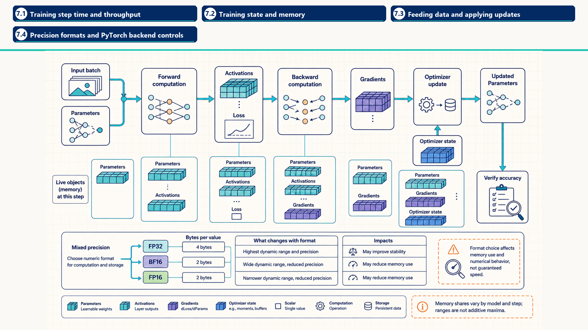
The diagram ties each memory object to the phase that uses it instead of adding unrelated peak percentages. Mixed precision can reduce traffic or use faster hardware paths, but some values may require wider accumulation or master state. The result must preserve stable learning and acceptable model quality, not only reduce step time.

The levers this chapter develops, in the vocabulary of Section 1.6.1, are fit in memory, because activation checkpointing trades arithmetic for resident bytes, use faster hardware paths, because mixed precision reaches the Tensor Core path, and keep the hardware busy, because the input pipeline decides whether the GPU waits.

7.1 Training step time and throughput

Training performance is the cost of repeating one parameter-update step. A batch is prepared and transferred, the model runs forward, backward propagation produces gradients, and the optimizer updates parameters. The slowest region or the uncovered gap between regions limits how many tokens can be trained per second.

• Training step: One repeated cycle that consumes a batch, computes a loss, propagates gradients, and updates model parameters.
• Step time: Elapsed time from the start of one training step to the start of the next comparable step after warmup. It includes data delivery, GPU work, optimizer work, and any communication that remains exposed.
• Global batch: All examples consumed before one optimizer update. On one GPU it is the local micro-batch (the examples processed by one forward and backward pass, Section 7.3) times gradient-accumulation steps. Across ranks it also includes the number of data-parallel replicas (full copies of the model on different GPUs).
• Training throughput: Useful training tokens or examples completed per second. It must be reported with global batch, sequence length, precision, and the quality or convergence condition.
• Exposed tail: Work that remains after useful overlapping work has finished. For a single GPU it can be an input, optimizer, or synchronization delay. In distributed training it often includes unfinished communication.

\[ \text{training step time} \approx \text{data pipeline} + \text{input transfer} + \text{forward} + \text{backward} + \text{optimizer} + \text{exposed communication} \tag{7.1}\]

To use this sum when phases overlap, count only each phase’s exposed contribution to the update interval, so no interval is counted twice. Summing the full durations is appropriate only for a serialized step. Input transfer can overlap with prior GPU work, and later distributed sections show how communication can overlap backward propagation. The useful diagnosis is the part that remains on the critical path after available overlap is accounted for.

The table below maps visible step symptoms to the first measurement that separates likely causes. It is a starting diagnosis, not a claim that one symptom has only one explanation.

Table 7.1: Training-step symptoms and first measurements.

Visible step symptom	Likely live object or gap	First measurement
GPU idle before forward	CPU batch preparation, storage reads, tokenization, or host-to-device transfer	Timeline with data-loader work, copy events, and the first GPU kernel
Peak memory rises through forward	Saved activations and temporary attention or workspace tensors	Peak allocated/reserved memory plus activation-lifetime inspection
Backward dominates step time	Gradient kernels, activation reads, or unfused reductions	Kernel timeline and arithmetic-intensity or memory-traffic counters
Update is unexpectedly expensive	Optimizer moments, parameter writes, or many small update kernels	Optimizer-region timing and memory-traffic profiling
Step ends with a long wait	Uncovered input, synchronization, or distributed communication	Timeline showing the final CPU/GPU or rank-to-rank dependency

The symptom table identifies where to measure first, but the limiting term is the work or gap that remains on the critical path after overlap. The next question is which parameters, activations, gradients, and optimizer buffers are live together and set the memory ceiling.

7.2 Training state and memory

Training usually keeps more live state than a weight-only inference baseline because a step holds gradients, optimizer buffers, and saved activations alongside parameters. A serving process can still exceed that baseline when long-lived KV cache, request state, and workspaces consume substantial memory.

State held during training

• Parameters: Learned values read during forward and updated by the optimizer. They persist across steps.
• Gradients: Derivatives produced during backward and consumed by the optimizer. Their values are step-specific. Their storage may be retained and zeroed, or released and recreated when gradients are set to None, such as with zero_grad(set_to_none=True).
• Optimizer state: Persistent update buffers such as Adam’s first and second moments.
• Saved activations: Forward intermediates kept only until backward has used them. Their size grows with micro-batch and sequence length.

Techniques that reduce different parts of that state

• Activation checkpointing: Saves fewer activations and recomputes selected forward regions during backward.
• Low-Rank Adaptation (LoRA): Freezes the base parameters and trains small adapter matrices, reducing trainable parameters, gradients, and optimizer state but not the required activations¹.
• Quantized Low-Rank Adaptation (QLoRA): Also stores the frozen base model in a quantized form, provided compatible dequantization kernels (which convert the stored low-bit values back to 16-bit for computation, Section 8.7.1) are available.

LoRA and QLoRA change which parameter tensors receive gradients. Activation checkpointing changes which forward tensors remain live. They solve different parts of the memory budget and can be combined when both trainable state and saved activations are limiting the step.

The first-order activation estimate separates linear saved tensors from a quadratic attention term. Let n_hidden count the retained hidden-sized tensors and n_score count the retained attention-score-like tensors in one layer. Those counts depend on the layer implementation, backward algorithm, and recomputation policy:

\[ \text{activation elements per layer} \approx n_{\text{hidden}} B T d + n_{\text{score}} B H T^2 \tag{7.2}\]

\[ \text{activation bytes} \approx b L (n_{\text{hidden}} B T d + n_{\text{score}} B H T^2) \tag{7.3}\]

Here B is the micro-batch size, T the sequence length, d the hidden dimension, H the attention-head count, b the bytes stored per element, L the layer count, n_hidden the retained hidden-sized tensor count, and n_score the retained attention-score-like tensor count. The formula exposes scaling. Measure the actual retained tensors to determine the runtime’s peak memory.

For a GPT-2 Large-style coarse estimate, set n_hidden = 16, n_score = 1, and use 36 layers, hidden dimension 1,280, 20 heads, sequence length 1,024, batch one, and two-byte activation storage. The linear and quadratic terms are then each about 21 million elements. Together they require about 84 MB decimal per layer and about 3.0 GB decimal across 36 layers in this first-order model. Increasing the batch to 32 raises the same estimate to about 96 GB decimal before optimizer state, workspaces, and allocator headroom.

The following choices reduce different live objects. They should be selected from the memory account, not treated as interchangeable capacity fixes.

Table 7.2: Training memory levers by the state object they reduce.

Memory lever	Object reduced	Main cost or condition
Activation checkpointing	Saved activations	Recomputes selected forward regions during backward and increases step compute
Smaller micro-batch with accumulation	Per-step activations	Needs more accumulation steps to preserve global batch; can change optimizer and scheduling behavior
BF16/FP16 or supported FP8 path	Stored activations, gradients, and selected state	Requires stable numerical behavior, compatible kernels, and correct accumulation or scaling policy
FlashAttention-style attention	Materialized attention-score-like tensors	Applies only when the selected attention kernel and dimensions are supported
State sharding	Per-rank parameters, gradients, or optimizer state	Introduces collectives and is developed after the communication foundations in Chapters 12 and 13

Activation memory and model-state memory are separate constraints. A sharding strategy can make a model fit while activations still exceed capacity. Checkpointing can lower activations while optimizer buffers remain the limiting state. A useful memory report names the largest live object at peak, not only total allocated bytes.

7.3 Feeding data and applying updates

Training-step speed depends on the complete path: the host prepares the next batch, copies move it to the GPU, forward and backward kernels execute, and the optimizer reads gradients and persistent state before the next step begins.

• Data pipeline: The CPU-side and storage-side path that reads examples, tokenizes or transforms them, assembles batches, and makes them available for GPU transfer.
• Micro-batch: The examples processed by one forward/backward pass before optional gradient accumulation. Its tensor dimensions determine activation memory and kernel shape.
• Gradient accumulation: Runs several micro-batches, adds their gradients, and performs one optimizer update afterward. It raises the effective global batch while keeping per-micro-batch activation memory lower.
• Fused optimizer: An optimizer implementation that combines update operations so parameters, gradients, and moment buffers are read and written with fewer launches or less intermediate traffic.

Accumulation preserves a chosen mean loss only when each backward pass contributes the correct fraction of that mean. For two equal-sized micro-batches with mean losses \(L_1\) and \(L_2\), the combined objective is \((L_1+L_2)/2\). Backward therefore uses \(L_1/2\) and \(L_2/2\), with parameters held fixed until both contributions have accumulated. Gradients are cleared before this cycle and after its single optimizer update, never between its backward passes².

Worked example: Two micro-batches, one update

Inputs and objective: Consider training a scalar model \(\hat y=\theta x\) with \(\theta=1\), inputs \(x_1=1\) and \(x_2=3\), and targets \(y_1=y_2=0\). Each one-example micro-batch has loss \(L_j=(\theta x_j-y_j)^2/2\). The intended objective is the mean over both examples. This illustrative calculation uses ordinary gradient descent with learning rate \(0.1\) and no momentum.

1. Clear old gradients. At the unchanged parameter \(\theta=1\), the losses are \(L_1=0.5\) and \(L_2=4.5\). Their derivatives are \((\theta x_j-y_j)x_j\), giving \(1\) and \(9\).
2. Backward on \(L_1/2\) leaves accumulated gradient \(0.5\). Backward on \(L_2/2\) adds \(4.5\), leaving \(5\). No optimizer update or gradient clearing occurs between them.
3. One combined batch also gives loss \((0.5+4.5)/2=2.5\) and gradient \((1+9)/2=5\). The optimizer applies \(\theta\leftarrow1-0.1(5)=0.5\) once, then clears the gradients for the next cycle.

Conclusion: Summing the two unnormalized gradients would give \(10\) and double this update. Matching the combined gradient assumes an additive objective and the same per-example forward behavior. Batch-dependent operations, random draws, and floating-point summation order can prevent exact agreement in a real model.

For an unweighted mean over valid training tokens, equal example counts need not mean equal loss weight. Let \(n_j\) count the non-ignored target positions in micro-batch \(j\), and let \(N=\sum_j n_j>0\) cover the whole accumulation cycle. If \(L_j\) is that micro-batch’s mean over its valid targets, its contribution is \((n_j/N)L_j\). Equivalently, each micro-batch’s summed valid-token loss is divided by the same \(N\). A micro-batch with no valid targets contributes zero without taking an empty mean. A shorter final accumulation cycle uses its actual count. A class-weighted or per-sequence objective requires its own reduction denominator. These counts and the following trace describe one worker. Distributed averaging must preserve the intended global objective as well.

Padding also affects throughput accounting. A valid training token here is a target position that contributes to the chosen token loss, after any target shift or mask. Padding and ignored targets do not count. For \(B_{\mathrm{global}}\) examples in a complete update, let \(n_i\) be example \(i\)’s valid-token count and \(t_{\mathrm{update}}\) the update duration in seconds, including all accumulated micro-batches:

\[ \text{useful training tokens/s} = \frac{\sum_{i=1}^{B_{\mathrm{global}}} n_i}{t_{\mathrm{update}}} \tag{7.4}\]

By contrast, \(B_{\mathrm{global}}T_{\mathrm{padded}}/t_{\mathrm{update}}\) counts processed tensor positions per second when all sequences are padded to length \(T_{\mathrm{padded}}\). It equals useful tokens/s only if every position contributes a valid target. Both rates use the same complete update boundary after warmup, with global batch, precision, and loss convention reported.

Worked example: Padding and useful throughput

Suppose two training sequences contribute 3 and 5 valid targets and are padded to a common length of 5. The complete update takes an illustrative 0.1 seconds. The loss mask excludes the two padded positions, so useful throughput is \((3+5)/0.1=80\) tokens/s. The tensor contains \(2(5)=10\) positions, giving \(10/0.1=100\) processed positions/s. Extra padding can raise the position count without adding training targets. The useful-token rate therefore answers how much loss-bearing data the update processed.

A change that also changes optimizer update frequency, the loss curve, or model quality creates a different training setup and must be evaluated separately.

Follow the training step in execution order and check each stage before tuning the next one:

1. Batch preparation: CPU workers, storage reads, tokenization, and collation make the next batch ready before the current GPU step finishes.
2. GPU transfer: Pinned host buffers, copy streams, and dependencies permit overlap without serializing the step.
3. Forward and backward evidence: Profiler evidence separates compute throughput, HBM traffic, launch overhead, activation memory, and gradient work.
4. Parameter-update evidence: Parameter, gradient, and optimizer-moment traffic are measured separately from backward. Supported runtimes can use fused update kernels.
5. Gradient accumulation: Preserves the intended effective batch while tracking gradient lifetime, memory use, update frequency, and synchronization.

These are single-worker training controls. Once the full step is understood locally, Chapters 12 and 13 add the communication and state-placement costs of scaling the same step across GPUs and nodes.

7.4 Precision formats and PyTorch backend controls

A numeric format determines how values use their available bits. In training, the format must preserve a stable update while reducing memory traffic and using efficient matrix hardware. In deployment, the same format choice can instead target model footprint or inference bandwidth.

A finite, nonzero normalized binary floating-point value has the form \((-1)^b(1.f)_2 2^e\). The sign bit \(b\) selects positive or negative. The exponent \(e\) sets the power-of-two scale. The significand \((1.f)_2\) holds the significant binary digits, with fractional bits \(f\) determining the spacing at a given exponent. Format descriptions often call these stored fractional bits the mantissa. The encoded exponent uses a bias to represent negative and positive exponents³.

Worked example: Range versus spacing

Assume a toy format with two fractional bits and allowed exponents from \(-2\) to \(2\). It describes normalized nonzero numbers only, omitting zero, subnormal numbers, infinities, and NaNs. The value \(+(1.10)_2 2^1=(1+1/2)2=3\) has positive sign, significand \(1.5\), and exponent \(1\).

At that exponent, adjacent values are \(2\), \(2.5\), \(3\), and \(3.5\): their spacing is \(2^1/2^2=0.5\). Rounding to the nearest value maps \(3.1\) back to \(3\), so adding \(0.1\) to a value stored as \(3\) can leave it unchanged. The largest positive value is \((1.11)_2 2^2=7\). A value of \(8\) lies outside this format’s range. Allowing a larger exponent would admit \(8\) but would not make the spacing near \(3\) finer. Adding a fractional bit would refine that spacing without adding another exponent.

Conclusion: Exponent range governs which magnitudes fit. Significand precision governs how closely nearby values can be distinguished.

This distinction explains the FP16/BF16 choice: BF16 covers a wider range but has fewer fractional bits than FP16. Loss scaling (multiplying the loss to reduce small-gradient underflow, defined below) can move small gradients into a representable range during backward, but cannot restore precision already lost to rounding or make a tiny update survive addition to a much larger low-precision weight. Wider optimizer state addresses that separate problem.

• FP32: 32-bit floating point. It is broadly supported and useful for numerically sensitive accumulation or reference results. The same tensor uses twice the storage of FP16/BF16. Operation speed depends on the GPU, TensorFloat-32 policy, dimensions, and selected library kernel.
• TF32: TensorFloat-32, an NVIDIA tensor-core mode for many FP32 matrix operations. It keeps FP32-like exponent range but uses a reduced mantissa, so it can be much faster than strict FP32 while being less precise.
• FP16: 16-bit floating point with smaller range than FP32. It is common for training and inference on tensor cores, but training may require loss scaling or mixed-precision practices to avoid overflow/underflow problems.
• BF16: 16-bit Brain Floating Point. It has FP32-like exponent range with fewer mantissa bits, which often makes training more stable than FP16 while still reducing memory traffic relative to FP32.
• FP8: 8-bit floating-point families used on newer accelerators with scaling metadata and compatible kernels⁴. Runtime support must handle scaling, accumulation, and selected operations.
• FP4 and block-scaled FP4: 4-bit floating formats often paired with one scale for a small block of values⁵. Block scaling can preserve local dynamic range, but it adds scale loads, packing constraints, and hardware-specific kernel requirements.
• INT8: 8-bit integer representation commonly used for quantized inference weights and sometimes activations (Section 8.7.1). It requires a mapping between integer codes and approximate real values, plus kernels that efficiently consume the representation.
• INT4: 4-bit integer representation often used for weight-only inference compression. Quality and speed depend strongly on grouping, scales, dequantization cost, and kernel support.
• Ternary weights: A specialized low-bit design whose weights take three values, such as negative, zero, and positive. It requires a model representation and kernel path designed for ternary values. An ordinary FP16 checkpoint needs conversion plus compatible kernels.

PyTorch precision settings permit framework-owned backend choices for supported operations. The selected path still depends on the PyTorch version, GPU, dimensions, dtype, and operation-specific eligibility. PyTorch 2.14 documents the newer precision controls and warns against mixing them with the older allow_tf32 flags in one configuration⁶.

Table 7.3: PyTorch precision controls and the conditions that determine their effect.

PyTorch control	Owner and scope	Performance meaning	Condition to verify
torch.backends.cuda.matmul.fp32_precision	PyTorch CUDA matrix policy in newer releases	Can permit reduced internal precision for supported FP32 matrix multiplication	Version, GPU support, output accuracy, and actual dispatched kernel
torch.backends.cudnn.fp32_precision	PyTorch cuDNN policy in newer releases	Can permit reduced internal precision for supported cuDNN operations	The operation is covered by cuDNN and the setting exists in the installed version
torch.backends.cuda.matmul.allow_tf32	Older PyTorch CUDA matrix flag	Allows TensorFloat-32 for supported matrix multiplication	Version-specific guidance and whether a newer control supersedes it
torch.set_float32_matmul_precision(...)	PyTorch matrix-multiplication API	Selects internal precision policy for float32 matrix multiplication	It does not control convolution precision or model-quality requirements
Scaled-dot-product attention backend policy	PyTorch attention dispatch	Permits flash, memory-efficient, or math attention paths	Device, dtype, mask, head dimension, sequence dimensions, and backend availability

The formats above describe available representations. The following update mechanisms keep reduced-precision compute paths numerically stable during training.

• Mixed-precision training: Runs selected tensor operations and storage in reduced precision while retaining higher-precision accumulation or selected state where numerical range matters⁷. The objective is lower traffic and faster matrix paths without destabilizing parameter updates.
• FP32 master weights: One common FP16 mixed-precision design keeps persistent FP32 parameters for optimizer updates and casts a reduced-precision compute copy for forward and backward kernels⁸. BF16, fused optimizers, sharded state, and newer low-precision recipes can use different layouts.
• Gradient underflow: A gradient becomes too small for the selected format and rounds to zero. FP16 is especially susceptible because its representable range is narrower than FP32 or BF16.
• Loss scaling: Multiplies the loss before backward propagation so small FP16 gradients are less likely to underflow, then divides the gradients by the same scale before the optimizer update⁹. Dynamic loss scaling lowers the scale after overflow is detected.
• Higher-precision accumulation: Accumulates reductions, dot products, or optimizer updates in a wider format than the input operands when the hardware and kernel path support it. This preserves numerical headroom while retaining much of the throughput benefit of reduced-precision inputs.

The mixed-precision state path separates the representation used by fast matrix kernels from the representation that receives the parameter update. A common FP16 path keeps FP32 master weights, uses loss scaling, then unscales and checks gradients before the FP32 update. BF16 has a wider exponent range and often does not need loss scaling, although the optimizer and accumulation layout still depend on the selected training stack.

\[ \text{scaled loss} = S \times \text{loss}; \quad \text{unscaled gradient} = \frac{\text{scaled gradient}}{S} \tag{7.5}\]

Here S is a positive loss scale. Scaling can keep small FP16 gradients representable during backward propagation, but one scale may still leave some gradients too small or make others overflow. Unscaling restores their intended magnitude before the optimizer updates the FP32 master weights. A finite-value check detects overflow before an invalid update is applied.

With gradient accumulation, the scale stays fixed through the whole cycle in Section 7.3. PyTorch automatic mixed precision (AMP) scales each normalized loss and accumulates the scaled gradients. Only after the last backward pass does it unscale, check for nonfinite values, and either apply or skip the optimizer update. Optional gradient clipping follows unscaling. In a one-optimizer PyTorch loop, scaler.step(optimizer) performs the check and unscales if needed, and scaler.update() adjusts the scale afterward. Clearing gradients then starts the next cycle¹⁰.

Worked example: Scaling an accumulated gradient

Using the two-micro-batch example from Section 7.3 with an illustrative fixed loss scale \(S=8\), the backward contributions are \(8(0.5)=4\) and \(8(4.5)=36\). Their sum is \(40\), and unscaling once gives \(40/8=5\), the intended combined gradient. Unscaling after the first contribution would instead mix \(0.5\) with the still-scaled \(36\). A single division could no longer recover the intended result. If the final accumulated gradients contain an infinity or NaN, the optimizer update is skipped and the scale is adjusted before the next cycle.

FP8 is a family, not one format. The two common FP8 encodings trade exponent range against mantissa precision, and practical systems add scaling metadata so tensors with wider dynamic range can still be represented¹¹.

The amax of a tensor is its maximum absolute element value, \(\max_i |x_i|\). An FP8 scaling recipe uses this magnitude, or a history of earlier magnitudes, to choose a scale that fits the tensor into the selected format. A large outlier can force coarser spacing for smaller values. Delayed scaling also depends on how well previous amax values predict the current tensor¹².

Table 7.4: FP8 format and scaling choices.

Format or scaling choice	What it changes	Performance effect
E4M3	Four exponent bits and three mantissa bits	More precision within a narrower range; often useful for values whose range can be controlled by scaling
E5M2	Five exponent bits and two mantissa bits	Wider dynamic range with less mantissa precision; useful when overflow risk is more important than small relative error
Per-tensor scale	One scale for a whole tensor	Low metadata overhead but poor fit when channels or blocks have different ranges
Per-channel or per-block scale	Separate scales for smaller groups	Better local fit and fewer saturated values, but extra metadata and more complex kernels

The same block-scaling idea appears in emerging FP4 paths. Transformer Engine 2.19 documents NVFP4, whose four-bit values use one sign bit, two exponent bits, and one mantissa bit (E2M1). Its one-dimensional format uses an E4M3 scale per 16-element block and an additional per-tensor FP32 scale. For comparison, MXFP8 stores eight-bit values, not four-bit values, and uses one E8M0 power-of-two scale per 32 values¹³. The local trade-off is scale precision against scale storage and conversion cost. These formats require compatible hardware and kernels. A reported FP4 throughput gain describes a particular model, accelerator, and runtime path, not a universal property of four-bit storage.

Performance condition

A smaller representation improves latency or throughput only when the runtime avoids moving the original wider values and uses an efficient hardware path for the selected format.

Bit width alone does not predict speed. During training, measure update stability and convergence. Deployment formats that store weights or the KV cache in fewer bits, and the quality checks they need, are the subject of Section 8.7.

Training changes parameters and therefore keeps gradients, saved activations, and optimizer state live. Inference fixes the parameters but introduces request state, prompt prefill, repeated token decode, and a growing KV cache. Chapter 8 builds that different workload and its user-visible metrics from the request path onward.

---

1. Hu, E. J., et al. (2021). LoRA: Low-Rank Adaptation of Large Language Models. arXiv:2106.09685. https://arxiv.org/abs/2106.09685. Supports freezing base weights and training injected low rank matrices to cut trainable parameters and memory, with no added inference latency after merging. Limit: reported parameter and memory reductions are for the paper GPT-3 style setup; activation memory still depends on micro-batch and sequence length.

2. PyTorch. (2.14 documentation). Automatic Mixed Precision examples, Gradient accumulation. https://docs.pytorch.org/docs/2.14/notes/amp_examples.html#gradient-accumulation. Supports fixed scaling during accumulation and unscale/check/step/scale-update at the effective-batch boundary. Limit: its equal-size example divides by the number of micro-batches; unequal valid-token counts require the objective-specific weighting derived here.

3. NVIDIA. (CUDA 13.4 documentation). Floating Point and IEEE 754, Sections 2.1-2.2. https://docs.nvidia.com/cuda/floating-point/index.html. Supports sign, biased exponent, fraction, finite precision, and rounding. Limit: the two-fractional-bit format is an illustrative calculation, not an IEEE format or hardware measurement.

4. NVIDIA. (Transformer Engine 2.19.0 documentation). Using FP8 and FP4 with Transformer Engine. https://docs.nvidia.com/deeplearning/transformer-engine/examples/fp8_primer.html. Supports E4M3 as 1 sign bit, 4 exponent bits, 3 mantissa bits up to about plus or minus 448, and E5M2 as 1 sign bit, 5 exponent bits, 2 mantissa bits up to about plus or minus 57344; the usual hybrid use is E4M3 for forward weights and activations and E5M2 for backward gradients, with one FP32 scale per tensor in current scaling. Limit: H100 and Blackwell Tensor Core support and recipe availability vary by GPU and Transformer Engine release; the chapter table keeps the choice as a measurement decision.

5. NVIDIA. (Transformer Engine 2.19.0 documentation). Using FP8 and FP4 with Transformer Engine. https://docs.nvidia.com/deeplearning/transformer-engine/examples/fp8_primer.html. Describes four-bit NVFP4 values of magnitude up to 6, a scale per 16 values, and an additional FP32 tensor scale. Its training recipe uses 16 by 16 scaling for weights. The eight-bit MXFP8 comparison uses a power-of-two scale per 32 values. These are Blackwell-specific recipes, not evidence of a universal speedup.

6. PyTorch. (2.14 documentation). CUDA semantics, TensorFloat-32 on Ampere and later devices. CUDA semantics. Describes backend and operator precision controls and the unsupported mixing of old and new settings. Eligibility and accuracy still depend on the operation and hardware.

7. Micikevicius, P., et al. (2018). Mixed Precision Training. arXiv:1710.03740. https://arxiv.org/abs/1710.03740. Supports storing weights, activations and gradients in FP16 with an FP32 master copy, scaling loss before backward and unscaling before update, and accumulating FP16 products in FP32. Limit: the method targets FP16 range limits; BF16 and FP8 paths in the chapter have different stability and kernel conditions.

8. Micikevicius, P., et al. (2018). Mixed Precision Training. arXiv:1710.03740. https://arxiv.org/abs/1710.03740. Supports storing weights, activations and gradients in FP16 with an FP32 master copy, scaling loss before backward and unscaling before update, and accumulating FP16 products in FP32. Limit: the method targets FP16 range limits; BF16 and FP8 paths in the chapter have different stability and kernel conditions.

9. Micikevicius, P., et al. (2018). Mixed Precision Training. arXiv:1710.03740. https://arxiv.org/abs/1710.03740. Supports storing weights, activations and gradients in FP16 with an FP32 master copy, scaling loss before backward and unscaling before update, and accumulating FP16 products in FP32. Limit: the method targets FP16 range limits; BF16 and FP8 paths in the chapter have different stability and kernel conditions.

10. PyTorch. (2.14 documentation). Automatic Mixed Precision examples, Gradient accumulation. https://docs.pytorch.org/docs/2.14/notes/amp_examples.html#gradient-accumulation. Supports fixed scaling during accumulation and unscale/check/step/scale-update at the effective-batch boundary. Limit: its equal-size example divides by the number of micro-batches; unequal valid-token counts require the objective-specific weighting derived here.

11. NVIDIA. (Transformer Engine 2.19.0 documentation). Using FP8 and FP4 with Transformer Engine. https://docs.nvidia.com/deeplearning/transformer-engine/examples/fp8_primer.html. Supports E4M3 as 1 sign bit, 4 exponent bits, 3 mantissa bits up to about plus or minus 448, and E5M2 as 1 sign bit, 5 exponent bits, 2 mantissa bits up to about plus or minus 57344; the usual hybrid use is E4M3 for forward weights and activations and E5M2 for backward gradients, with one FP32 scale per tensor in current scaling. Limit: H100 and Blackwell Tensor Core support and recipe availability vary by GPU and Transformer Engine release; the chapter table keeps the choice as a measurement decision.

12. NVIDIA. (Transformer Engine 2.19.0 documentation). Using FP8 and FP4 with Transformer Engine. https://docs.nvidia.com/deeplearning/transformer-engine/examples/fp8_primer.html. Supports E4M3 as 1 sign bit, 4 exponent bits, 3 mantissa bits up to about plus or minus 448, and E5M2 as 1 sign bit, 5 exponent bits, 2 mantissa bits up to about plus or minus 57344; the usual hybrid use is E4M3 for forward weights and activations and E5M2 for backward gradients, with one FP32 scale per tensor in current scaling. Limit: H100 and Blackwell Tensor Core support and recipe availability vary by GPU and Transformer Engine release; the chapter table keeps the choice as a measurement decision.

13. NVIDIA. (Transformer Engine 2.19.0 documentation). Using FP8 and FP4 with Transformer Engine. https://docs.nvidia.com/deeplearning/transformer-engine/examples/fp8_primer.html. Describes four-bit NVFP4 values of magnitude up to 6, a scale per 16 values, and an additional FP32 tensor scale. Its training recipe uses 16 by 16 scaling for weights. The eight-bit MXFP8 comparison uses a power-of-two scale per 32 values. These are Blackwell-specific recipes, not evidence of a universal speedup.