Appendix A — Execution records and supporting notebooks
Reference records separate local checks, historical outputs and full experiments, retaining their data, versions, settings and missing execution.
A numerical check, a full experiment and a historical notebook output support different claims. This reference keeps their environment, data and execution records accessible without interrupting the mechanism explanations. Chapter 24 contains the task-specific comparisons.
A.1 Environment and notebook status
An experiment cannot be reproduced from a model name and final score alone. Its record needs the Python and package versions, operating system, device, driver and accelerator runtime when used, seeds, and numerical types. Retain model and tokenizer revisions, data version, split construction, preprocessing, training settings, and decoding choices. A seed does not guarantee identical results across different hardware or kernels.
| Supporting notebook | Teaching role |
|---|---|
| PyTorch basics | Tensor creation, layout, indexing, and numerical practice |
| Gradients and logistic regression | Manual derivatives and a training loop |
| Word embeddings | Corpus fitting, vector queries, and projection inspection |
| Logistic regression and optimizer comparison | SST-2 and optimizer comparisons, §24.1 |
| Text classification and recurrence | AG News classification and Character LSTM labs, §§24.2 and 24.5 |
| Attention and fine-tuning | Controlled heads and audience adaptation, §§24.3–24.4 |
| N-gram language modeling | Counts, generation, and reload, §24.6 |
| Multimodal inference | Captioning and visual questions, §24.7 |
| PyTorch on GPU | Device and kernel experiments under their original environment |
To compare initializations, use reproducible random seeds and hold the data, architecture, optimizer, and update budget fixed. Record activation ranges, gradient behavior, and validation results. A seed controls the random generator it initializes. Repeatability also depends on the software, hardware, and operations used. Neither a seed nor a repeated result establishes that one initialization is better.1
The downloadable notebooks are unchanged snapshots of the supplied files. Their outputs are historical source results, not results of the code in this book. Open them in an existing compatible notebook environment and inspect dependencies before execution. A package installed for one notebook does not establish compatibility with every other model path.
Unless a listing selects otherwise, floating-point tensors use float32 on the CPU. Integer ID and class-index label tensors use int64. The API references for these listings cite PyTorch 2.12. An execution record must identify the version that actually ran. These listings need no large model downloads. Full experiments may require datasets, pretrained weights, network access, or supported accelerator hardware. When unavailable, retain the failed step and its cause as unexecuted work rather than substituting a toy result.
The record connects inputs, intermediate arrays, parameter changes, metrics and errors. It maps mathematical objects to code objects, axes, dtype and device. Retained plots need titles, labeled curves and common comparison scales. Executed and unavailable branches have separate results and status fields.
A.2 Historical tensor and embedding notebooks
The original notebook settings identify their recorded calculations. Reusing a seed without the same input and sequence of draws does not reproduce a later array.
The PyTorch basics notebook supplies tensor creation, seeds, indexing, and reshaping practice. Its recorded sequence uses seed 8436, Gaussian samples with mean zero and standard deviation two, uniform samples from negative two to two, and 500 Poisson draws with rate one. Reproducing a later random sample requires the preceding draws as well as the seed because each draw advances the generator state. Its torch.Tensor(1000) allocation is uninitialized and must be filled before its values are used. A ten-bin histogram over values from zero through ten displays only the draws in that range. The Poisson distribution can still produce larger values. These are array-generation checks, not measured neural initialization results.
The word-embedding source notebook describes fitting CBOW vectors with min_count=100, window=5, and vector_size=100 on roughly 25,000 computational-linguistics abstracts collected before mid-April 2021. Its /content/arxiv.csv corpus is not bundled, so reproducing the recorded neighbors requires that data or a declared replacement. Its inspection prompts compare nmt with smt and ner, retrieve neighbors of bert, query transformer + lstm - bert, and compare tree with tree - syntax. Record the corpus, preprocessing, vocabulary, Gensim version, settings, query, and seed with any result. The separate three-sentence check in §14.2 uses Gensim 4.4.0, Skip-gram, and supplied local text.
A.3 Accelerator availability and timing boundary
The source notebook includes a device inventory and a specific matrix-vector workload. Its historical ratios are separate from a new timed run.
An accelerator comparison first needs to establish which device can run the calculation. In the optional GPU notebook, check torch.cuda.is_available() and torch.cuda.device_count() before choosing a CUDA device. For a selected available device, record get_device_name(device), get_device_capability(device), and memory_allocated(device) from torch.cuda. These report the hardware name, compute-capability version, and bytes currently allocated to tensors. Compute capability identifies a CUDA hardware feature version used to check instruction and compiled-kernel compatibility. It is not a measured speed or a count of cores. They are separate from total device memory. If CUDA is unavailable, record that condition and use a declared CPU comparison or leave the accelerator run unexecuted.
The matrix-vector workload uses a float32 matrix with 100,000 rows and 100 columns, and a vector of width 100. The PyTorch and NumPy timing cells specify 100 loops and three repeats. The NumPy inputs are copied to the CPU before its timed np.dot call. The notebook reports historical ratios of about nine for an earlier comparison compiled with Numba, a Python compiler for numerical functions, and about 100 for PyTorch against NumPy. These ratios describe that hardware and measurement setup. A new result requires the synchronization, transfer boundary, and repeated-accumulation checks in §23.5. The notebook also contains kernel implementations for separate study. Kernel tuning is outside the scope of this book.
A.4 Generation and serving interfaces
Chapter 21 explains cache identity, request state and physical allocation. These interfaces connect those mechanisms to specific implementations. Their availability and behavior need a versioned environment record.
The transformers method model.generate manages model calls and selection for a local generation interface. vLLM, SGLang, and TensorRT-LLM are serving implementations that organize requests, caches, and accelerator execution.
For a scoped historical interface example, vLLM 0.10.2 documents --enable-prefix-caching. It is an engine flag rather than a generic transformer operation.2 No installed engine or running flag configuration is implied here. Changing kernels or numerical formats can affect computed scores even when the intended mathematical model stays the same.
A.5 Additional target-alignment shapes
The width-four update in §20.8 calculates actual loss gradients. This separate width-64 case checks only the target layout and vocabulary-head dimensions.
Use the recorded tokens The cat sat on, with IDs \([1,2,3,4]\). Choose three input positions \([1,2,3]\) and their following labels \([2,3,4]\). The fourth recorded token supplies the extra target. The example vocabulary has \(|V|=5000\) entries and model width \(D=64\).
For \(B=1\) and \(T=3\), the input and manually aligned labels both have shape \([1,3]\). Hidden representations have shape \([1,3,64]\). A vocabulary matrix stored as \([5000,64]\) maps them to logits \([1,3,5000]\). The loss includes the three target positions in this example.
The four recorded tokens supply three next-token comparisons. Their mean loss averages those three included target penalties, using §8.5’s loss calculation. Cross-entropy uses the target’s normalized log probability. Its normalization depends on the entire vocabulary-score row, not only the target logit. If a loss mask retains only \(N_{\mathrm{tgt}}>0\) targets, the sum and divisor instead use those \(N_{\mathrm{tgt}}\) positions.
Under §8.5’s model-internal shift, the full four-token input and copied labels form these same three comparisons. Section 20.8 follows the gradients into the adapter parameters.
A.6 Original NLTK corpora and generation settings
The local two-sentence example in §24.6 checks counting, persistence and generation. The source tutorial uses different corpora and preprocessing, recorded here for a separate reproduction.
The tutorial first uses two unequal sentences, ['a','b','c'] and ['a','c','d','c','e','f']. Inspect unpadded bigrams of the first sentence and trigrams of the second to expose the different history lengths before boundary markers are added. Inspect the first sentence with one marker at each end for bigrams and two for trigrams. Then inspect everygrams up to length two and flatten both bigram-padded sentences for the vocabulary stream. Finally, materialize each training sentence’s n-gram iterator and the vocabulary iterator from padded_everygram_pipeline(2, text). Recreate both iterators before fitting. These inspections explain what is counted. They do not pad the unequal sentences into a dense tensor batch.
The downloadable tutorial fits its first trigram model to the prose file language-never-random.txt. It reads an existing UTF-8 cache or downloads and saves the pinned text linked by the source. Its tokenizer check first tries NLTK sentence and word tokenization. The fallback uses a regular-expression sentence splitter and ToktokTokenizer. It lowercases the prose tokens before fitting. Record which tokenizer path ran, inspect the first 500 raw characters beside the first tokenized sentence, and retain the resulting tokens. A fallback can change the counts even when the downloaded text is unchanged.
For the tutorial’s prose model, apply model.vocab.lookup to its first tokenized sentence as the known example, and to language is never random lah . split into words as the mixed known/unknown example.
Inspect model.counts before querying individual entries. For the tutorial’s fitted prose model, model.counts['language'] retrieves a unigram count. model.counts[['language']]['is'] retrieves a continuation count after one word, and model.counts[['language','is']]['never'] after two. Compare these raw counts with model.score('language'), model.score('is', ['language']), and model.score('never', ['language','is']): the scores divide by the total count for the relevant history. Check that the no-history scores for unseen lah, leh, and lor equal the score for <UNK>. The vocabulary performs that mapping before scoring. Equality does not imply a positive probability. These source-corpus inspections are separate from the two-sentence calculation above.3
The second corpus comes from the Tweet_Text column of Donald-Tweets!.csv, obtained through the source’s tweet dataset archive. Load the CSV with pandas.read_csv and inspect df.head() to check its table and text column before tokenization. This corpus uses the selected word tokenizer without the prose lowercasing step and fits a separate trigram model. Retain casing, tokens and vocabulary with each corpus. Historical notebook outputs are tied to those original data and preprocessing choices. A replacement corpus requires a separate record rather than an implied reproduction.
The tutorial’s generation calls omit text_seed, so they begin with an empty history and sample the first token from the fitted unigram counts. The local example above instead supplies two start markers. Its generated output is therefore a separate conditional experiment. The source helper generate_sent(model, num_words, random_seed=42) skips generated <s> markers, stops at the first </s>, and detokenizes the retained tokens. The tutorial saves the prose model to kilgariff_ngram_model.pkl with dill and reloads that file before its repeat generation. This disk save/load path differs from the local example’s in-memory round trip. Preserve the tutorial’s prose (token budget, random seed) cases (20,7), (28,0), (20,1), (20,30) and (20,42), including (20,42) after saving and loading. Preserve its tweet cases (40,42), (10,0), (50,10) and (100,52). The source pairs raw tokens and cleaned text for its prose (20,7) and (28,0) cases. For additional diagnosis, retain both forms for the other cases too. The token budget limits draws, while the text helper stops at the first end marker. That can produce an empty displayed string. Neither a fixed seed nor a larger budget guarantees a complete sentence.4
A.7 Evidence retained for an experiment
The classifier result in §24.8 distinguishes its executed update from unmeasured task quality. A fuller comparison needs the following evidence in addition to a local assertion.
The resulting evidence should contain five connected elements:
- An environment and data record, including the held-out boundary and actual computation budget.
- One small input traced through intermediate arrays to an independently checkable numerical result, with the relevant shapes, masks, dtype, reduction, and expected values. A training trace includes a derivative or parameter update. An inference trace includes selection and changing state.
- A baseline and one change executed under the same evaluation protocol. Actual training or inference results remain separate from local assertions. An unavailable run stays unexecuted, with its missing dependency identified.
- Contrasting outcomes or errors that show what the results support and which proposed causes remain uncertain. A performance claim additionally needs the timing boundary and hardware record from §23.5.
- A configuration choice justified by the task criterion and resource cost, together with missing evidence that could change the choice and enough input-output records for another reader to inspect the conclusion.
The differentiation illustration applies when the experiment includes training. Inference-only comparisons instead follow fixed parameters and changing input or request state.
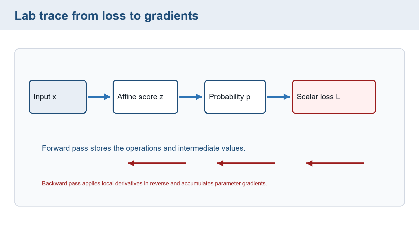
The record identifies which branches ran, which failed, and which remain unavailable. A planned procedure has no measured outcome until it is executed.
PyTorch Contributors. (2026). Reproducibility. PyTorch 2.12 documentation.↩︎
vLLM Contributors. (2025). Engine arguments. vLLM 0.10.2 documentation. The page documents the engine-specific option and does not establish a current installed configuration.↩︎
NLTK Project. (2025). Language-model API. NLTK 3.9.2 source,
logscore,entropy,perplexity, andgenerate.↩︎NLTK Project. (2025). Language-model API. NLTK 3.9.2 source,
logscore,entropy,perplexity, andgenerate.↩︎