Roadmap
The book follows how data becomes a model input, how a calculation produces a prediction, and how training can change that calculation. The distinctions between inference, training, and evaluation introduced in Foundations determine which calculations each task requires.
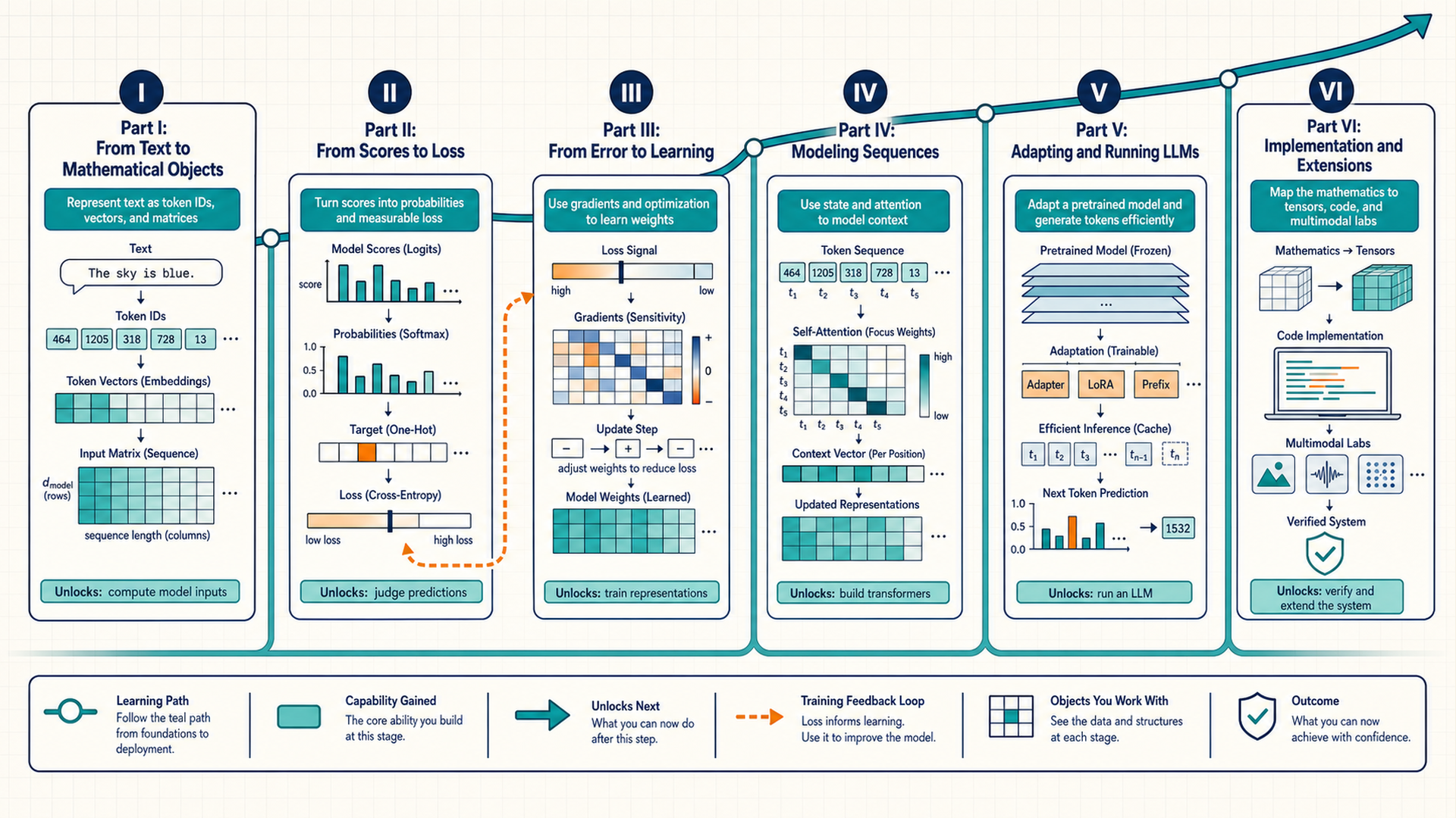
The six Parts organize learning dependencies. Two representation routes share the task definitions: document features can feed a classifier, while ordered token IDs can select vectors for a sequence model. Neither representation must pass through the other.
- Part I: From Text to Mathematical Objects, Chapters 1–4. Inputs, targets, token IDs, batches, subwords, and fixed feature coordinates.
- Part II: From Scores to Loss, Chapters 5–9. Affine predictions, local derivatives, probabilities, inference choices, loss, and held-out evaluation.
- Part III: From Error to Learning, Chapters 10–14. Parameter updates, gradient propagation, nonlinear models, and learned token vectors.
- Part IV: Modeling Sequences, Chapters 15–19. Limited history, recurrent state, attention, transformer families, and pretraining.
- Part V: Adapting and Running LLMs, Chapters 20–21. Adapting a pretrained model and managing generation state.
- Part VI: Implementation and Extensions, Chapters 22–24. Other input modalities, tensor storage, and computational labs.
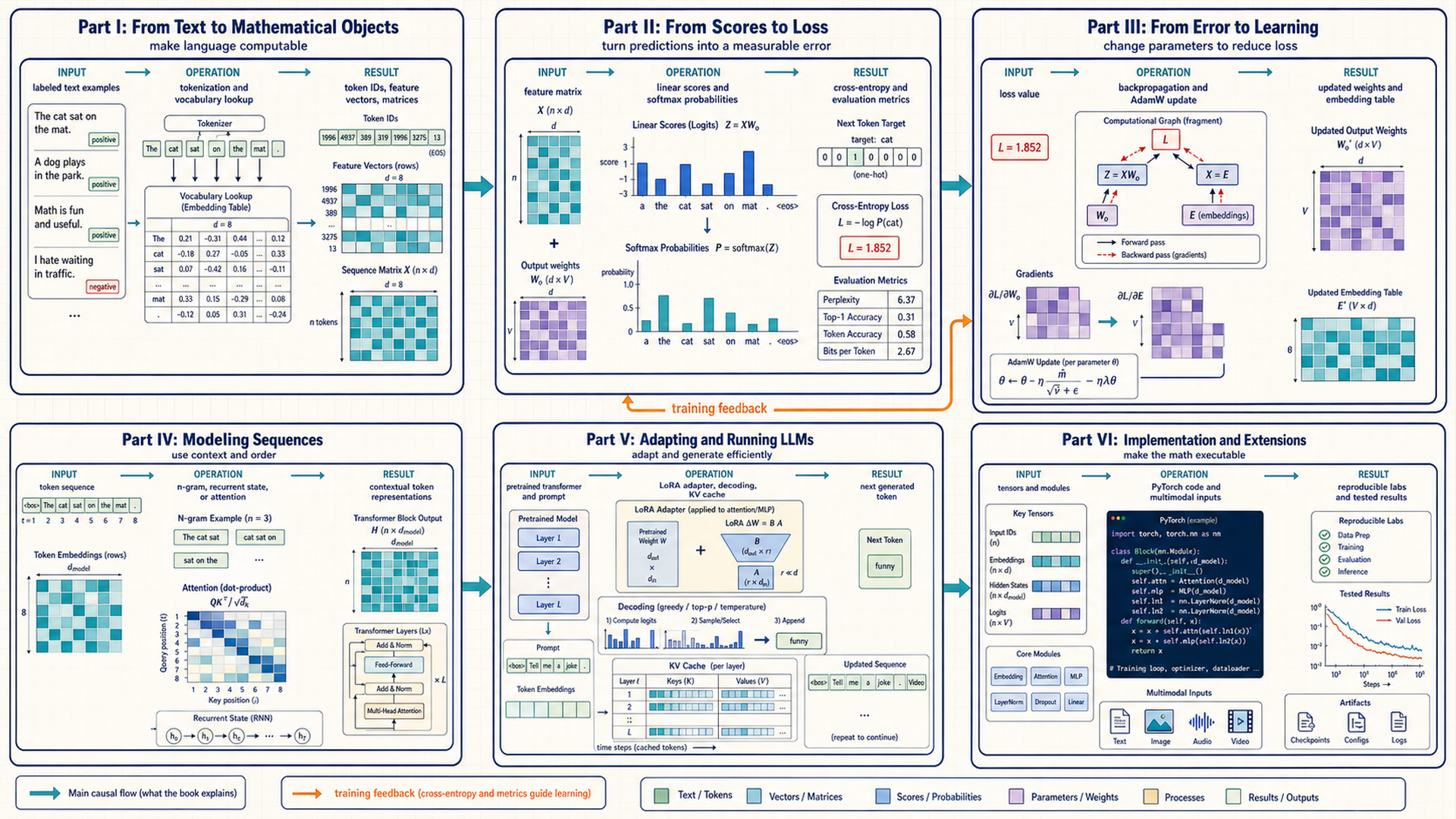
The arrows relate prerequisites. Later chapters use fixed parameters during decoding, compare predictions with learning targets during training, or measure fixed-model behavior against task criteria during evaluation, as the local calculation requires.
The second map connects representation, prediction, learning, sequence context, serving, and implementation. These are related study routes, with the task determining which operations are required.
Foundations distinguishes tasks, model families, and learning settings. Four choices remain separate throughout: the required result, the model structure, the training objective, and the inference procedure. For example, next-token targets differ from selected masked-token targets, and sequence-to-sequence tasks specify an output sequence for an input sequence. Representation learning instead shapes vectors for uses such as similarity and retrieval. A task’s output form does not select its model family automatically.
The family comparison below is a lookup aid to the later mechanisms. A recurrent model uses the preceding hidden state when processing the next sequence position. Attention combines information from permitted positions. Vision and multimodal models first convert images, audio, or other inputs into suitable vectors.
| Family | Context used | Typical output | Chapters |
|---|---|---|---|
| Linear and logistic models | A fixed feature vector | A number or one class | 5-6, 9 |
| N-gram models | A fixed token history | A next-token probability | 3.4, 15.1 |
| RNNs and LSTMs | A recurrent hidden state | Sequence labels or generated tokens | 15 |
| Transformers | Attention over permitted positions | Classes, tokens, or a target sequence | 16-21 |
| Vision and multimodal models | Patches, frames, fields, or text vectors | A label, matched pair, or generated text | 22 |
The inputs, model parameters, intermediate results, and training state have different roles and storage costs. Chapter 23 brings these objects together after their calculations have been introduced.
Starting knowledge and tensor notation
This book is for software engineers and technically trained readers who want to understand the calculations behind language-model training and inference. It assumes school-level algebra, functions, averages, summation notation, and familiarity with scalars, vectors, and matrices. Basic probability and the ability to follow Python lists, indexing, functions, and imports are also assumed.
Machine-learning concepts are introduced as they become necessary. The book explains prediction tasks, loss, empirical risk, gradients, attention, and their practical consequences. It uses familiar mathematics directly while explaining what each quantity and operation means for the model. The derivative, gradient, and chain-rule foundation is taught in §5.4. Chapter 11 extends it to automatic differentiation through a graph, including the operations exposed by PyTorch. Readers who need a reminder of matrix multiplication can use the dimension calculation in §5.3 before continuing to embeddings and attention.
A tensor is an array with explicit axes, a numerical type, and a storage device. An array with dimensions \([B,T,D]\) contains \(B\) examples, \(T\) positions per example, and \(D\) coordinates per position. For \([2,3,4]\), there are \(2\cdot3\cdot4=24\) values. Integer token IDs select rows, floating-point arrays hold learned vectors, and Boolean arrays can mark permitted positions. The device identifies where the array is stored and computed, such as central processing unit (CPU) memory or a graphics processing unit (GPU). CUDA is NVIDIA’s software and device platform through which the PyTorch examples can select a supported GPU, such as device cuda:0.
Matrix multiplication sums over a shared axis. For example, multiplying dimensions \([B,F]\) by \([F,D_{\mathrm{out}}]\) removes the shared feature axis \(F\) and produces dimensions \([B,D_{\mathrm{out}}]\). §5.3 presents the calculation and the orientation used by nn.Linear. Chapter 23 later develops storage, strides, copies, and device costs.
Reading paths and scope
Read Chapters 1–6 for targets, representations, and probability outputs. From there, Chapter 7 follows inference with fixed parameters. Chapter 8 develops losses, Chapter 9 evaluation, Chapter 10 update rules, and Chapter 11 gradient propagation. The default path already has the calculus foundation from §5.4 before probability and loss derivatives rely on it. Readers who prefer derivation before optimizer comparisons can read Chapter 11 before Chapter 10.
For text classification, read the loss and evaluation foundations in Chapters 8–9 and the update and gradient calculations in Chapters 10–11. Then continue through nonlinear classifiers, embedding lookup, and Word2Vec in Chapters 12–14 before the classification lab. For the count-model route, begin with n-gram counts and smoothing, read logarithmic loss and perplexity in §§8.1 and 8.5, then continue to the count-model lab. These establish the baseline before recurrent state, attention, and transformers. For adaptation and serving, complete Chapters 17–21 before the QLoRA lab. The multimodal lab examines image representations, captioning, and visual question answering.
The book develops the mathematics behind the supplied LLM Architecture lectures and notebooks, with tensor examples from Python for Data Processing, Lecture 3. References to the course mean these source materials unless another course is identified. It explains the objects and calculations needed to inspect training and inference: tensor dimensions, probabilities, gradients, attention, adapters, and cache storage. Kernel programming, Tensor Core scheduling, memory coalescing, production benchmarking, and complete distributed training configurations are outside this book’s scope. Mixed precision and serving engines appear only where they change a mathematical assumption, memory estimate, or experimental choice.
References and execution guidance
Use the notation reference to check symbols, dimensions, and mask conventions. The library map connects each operation to its first introduction and practical exercise. The Glossary expands abbreviations and returns to the section that explains them.
Each code example states its scope. A runnable calculation checks the listed inputs and outputs. An abbreviated fragment requires the surrounding model or data objects. A course experiment additionally needs its dataset split, checkpoint, training configuration, and held-out results. Passing a tensor assertion establishes neither model quality nor a speed improvement. The Environment and source notebooks explains the environment and evidence to retain.
The References collect the sources cited beside the explanations.