1  SFT for task responses

A pre-trained model can produce plausible text without consistently following a task’s format or constraints. Supervised fine-tuning (SFT) uses trusted prompt-response examples to make those demonstrated responses more likely. Demonstrated text becomes recorded token probabilities and a supervised update. SFT directly rewards reproducing its supplied answers, so later methods add comparisons or outcome evidence when the task needs more.¹

• Pre-trained language model: A model trained to predict the next token in internet-scale text. It has broad linguistic and factual capability, but it does not yet have task-specific evidence about which valid response best serves a user.

• Supervised Fine-Tuning (SFT): Training that continues from the pre-trained model using trusted prompt-response examples. It increases the probability of the demonstrated response, making the formats, tones, and skills shown in those examples more likely.

Post-training changes how that same model responds to prompts used in deployment. SFT, preference optimization, and online reinforcement learning use different evidence. They are not compulsory stages in one training chain.

A trusted answer must become token probabilities before it can train the model. The three steps below connect the choice of demonstration data to scoring the recorded answer and updating the model.

Figure 1.1: Recorded answer tokens supply the SFT training targets.

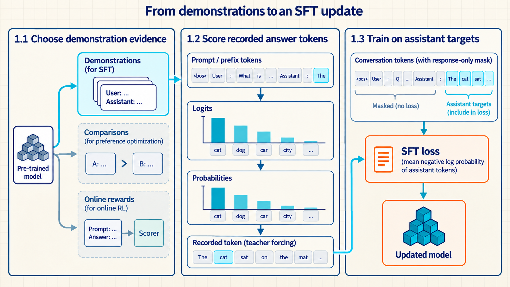
Follow Sections 1.1 to 1.3 from left to right. The highlighted recorded token is a training target, not a newly sampled answer. Only assistant response positions contribute to the illustrated loss. The update changes model parameters.

1.1 From pre-training to task behavior

Consider a model that can explain a test failure but returns a long essay when the task requires one diagnosis and one next step. Pre-training supplied broad language patterns, not this task’s response contract. SFT supplies trusted examples of that contract. A project may stop after SFT, use preference training without later PPO, or use online rewards when newly generated attempts must be scored.²

A pre-trained model may know many facts and still choose the wrong format, overlook a constraint, or select a plausible but inferior response. Post-training supplies evidence about which response behavior serves this task. It updates the same model parameters that support earlier capabilities, so improving the target behavior can also change or weaken another skill. Held-out evaluation must check both the intended improvement and those possible regressions.³

The following methods answer different training questions.

• Pre-training: Next-token likelihood builds language, world regularities, and broad skills, but does not provide task-specific evidence of helpfulness.

• SFT: One target completion for each prompt makes its instruction format, tone, and demonstrated skills more likely, but treats that one sample as the only target.

• Preference optimization: A chosen-versus-rejected pair identifies relative quality and alignment, but the quality signal is only as good as the comparison or reward behind it.

• RL for reasoning and agents: A learned, human, or verifier reward can shape multi-step behavior toward an outcome, but reward design can distort the behavior it reinforces.

The available evidence determines which method fits the task.

• Demonstrations: Use SFT when one clear answer is enough to show the required behavior.

• Comparisons: Add preference evidence when the important distinction is which of two acceptable-looking answers is better.

• Online rewards: Use online rewards when the current policy must generate new attempts and a scorer can evaluate them reliably.

Richer feedback requires different stored values, numerical quantities to optimize, and software components.

1.2 Computing probabilities for text

To make a trusted answer more likely, the trainer needs a number that says how probable its recorded tokens already are. The LLM policy \(\pi_\theta\) is the complete next-token decision rule, while \(\pi_\theta(y\mid x)\) is the probability it assigns to one exact answer. To calculate that score, hold the prompt and current text prefix fixed, normalize the model’s raw scores into a next-token distribution, select the probability of each recorded token, and combine the selected values into one answer score.

• LLM policy \(\pi_\theta\): The symbol \(\pi_\theta\) names the LLM’s complete decision rule, with \(\theta\) denoting its trainable weights. For one text state \(s_t\), \(\pi_\theta(\cdot\mid s_t)\) is the full next-token probability distribution returned by that rule. Selecting candidate token \(a_t\) gives the scalar \(\pi_\theta(a_t\mid s_t)\). Repeating the calculation for every recorded answer token and multiplying the selected values gives \(\pi_\theta(y\mid x)\) for one exact answer \(y\) after prompt \(x\).

The policy is the complete rule. A policy probability is one output of that rule. The numerical calculation begins by fixing exactly what text the LLM can see before it chooses the next token.

• Current text state \(s_t\): The prompt \(x\) plus the answer tokens already present before token step \(t\). The state is the complete text input used for the next-token calculation at that step.

A tokenizer splits text into vocabulary pieces and assigns each piece an integer token ID. A forward pass applies the model weights \(\theta\) to those IDs for the fixed state and returns one raw score for every vocabulary token. These raw scores are logits. They do not yet sum to one and are not probabilities.

• Softmax: At token step \(t\), the model returns a logit vector \(z_t\) with one raw score for every vocabulary token. Softmax exponentiates and normalizes that vector into non-negative next-token probabilities that sum to one. Training then selects the probability assigned to the recorded token.

• Policy output \(\pi_\theta(\cdot\mid s_t)\): The complete probability vector produced after softmax for state \(s_t\). The dot represents every candidate token in the vocabulary. Selecting the entry for candidate token \(a_t\) gives \(\pi_\theta(a_t\mid s_t)\), one scalar probability between zero and one rather than the policy itself.

The calculation therefore separates the model weights, the full distribution they produce, and the one value used to score a token. Repeating it at the recorded answer positions supplies the factors used to calculate \(\pi_\theta(y\mid x)\). The vertical bar means “given.”⁴

\[ \pi_{\theta}(a_t \mid s_t) = \frac{\exp(z_t[a_t])}{\sum_{j\in V}\exp(z_t[j])} \tag{1.1}\]

Variables

• \(\pi_\theta(a_t\mid s_t)\): Scalar probability assigned to candidate token \(a_t\) in state \(s_t\).
• \(\theta\): All LLM weights used by the forward pass. Post-training changes some or all of these numerical parameters.
• \(t\): Index of the current answer position.
• \(s_t\): Prompt plus the response prefix already present at token step \(t\).
• \(a_t\): Candidate next token being selected or scored.
• \(\pi_\theta(\cdot\mid s_t)\): Complete normalized probability vector returned for state \(s_t\).
• \(z_t\): Logit vector returned by the model for state \(s_t\).
• \(z_t[a_t]\): Raw logit assigned to candidate token \(a_t\).
• \(V\): Set of all token IDs in the model vocabulary.
• \(j\): One vocabulary-token index in the denominator.
• \(\exp\): Base-\(e\) exponential applied to a logit before normalization.

Mechanism: Exponentiation makes each logit contribution positive. The denominator sums those values. Division returns the selected token’s normalized share. Interpretation: Calculate one next-token probability between zero and one, with all vocabulary-token probabilities summing to one.

Example: softmax turns logits into a token probability

At one fixed prompt and response prefix, a toy model has token IDs 0, 1, and 2 with logits 2, 1, and 0 in that order.

Inputs and measurement

One policy forward pass returns one raw logit for every token in this three-token toy vocabulary. Softmax exponentiates and normalizes all three values. The trainer then reads the share assigned to token ID 0.

Calculation

1. Selected-token probability: \(\pi_\theta(a_t=0\mid s_t)=e^2/(e^2+e^1+e^0)=0.665\).

Interpretation: Token ID 0 receives probability 0.665, or 66.5 percent of the probability mass. The other token probabilities are approximately 0.245 and 0.090, so the three values sum to one. Generation can sample from them, while training can score a recorded token without sampling.

• Nat: The unit used for information quantities calculated with the natural logarithm \(\ln\). Using logarithm base 2 gives bits instead. A log probability and its negative-log loss have opposite signs, even though both use the same logarithm.

Applying \(\ln\) changes the numerical representation. It does not replace the original probability. For \(p=0.5\), the probability remains 0.5, its log-probability is \(-0.693\), and the corresponding negative-log loss is \(0.693\).

\[ p = 0.5, \ln p = -0.693, -\ln p = 0.693 \tag{1.2}\]

Because \(\ln\) is used, the two logarithmic values may be described as \(-0.693\) nats and \(0.693\) nats. A log-probability is at most zero and moves closer to zero as the text becomes more likely. Its negative is the non-negative value commonly used in training losses.

• Teacher-forced scoring: A controlled scoring pass for a fixed prompt and written answer. The recorded answer tokens are supplied to the model. No replacement answer is sampled.

A full-answer probability is one score derived from the policy, not a second policy. For fixed prompt \(x\) and complete answer \(y\), teacher forcing supplies the recorded answer rather than sampling a replacement. A causal model reads the prompt and shifted answer prefix. The logit row before each recorded token scores that token. One forward pass normally returns all of those rows at once. Multiplying the selected probabilities gives \(\pi_\theta(y\mid x)\), while summing their logarithms gives the stable answer score used in training. Here \(y\) includes the model’s end or stop token, so the result is the probability of the complete sequence. If the stop token is omitted, the product describes only the recorded prefix.⁵

\[ \pi_{\theta}(y \mid x) = \prod_{t=1}^{T}\pi_{\theta}(y_t \mid x, y_{<t}) \tag{1.3}\]

Variables

• \(\pi_\theta(y\mid x)\): Scalar probability assigned to the exact complete answer \(y\) after prompt \(x\).
• \(\pi_\theta\): The same next-token policy, evaluated at every answer position.
• \(\theta\): LLM weight values held fixed while this answer is scored.
• \(x\): Prompt held fixed while the answer is scored.
• \(y\): Complete written answer.
• \(t\): Answer-position index from 1 through \(T\).
• \(y_t\): Answer token at position \(t\).
• \(y_{<t}\): Answer prefix before token \(t\).
• \(T\): Number of tokens in \(y\).

Mechanism: Each factor is the probability of the recorded next token given the prompt and earlier recorded answer tokens. The product chains all \(T\) decisions. Interpretation: Calculate the probability of producing that exact token sequence. Longer answers usually have smaller raw products. Summed log-probabilities represent the same product stably. They do not by themselves make whole-answer comparisons fair across lengths. Scale: The product is a probability. Applying the natural logarithm produces a log score reported in nats.

Example: token probabilities become one answer score

A fixed three-token answer receives next-token probabilities 0.50, 0.40, and 0.20 under one policy.

Inputs and measurement

Teacher forcing runs the recorded answer through the model, applies softmax at each position, and gathers the probability of each recorded token ID.

Calculation

1. Completion probability and log score: The completion probability is \(0.50\times0.40\times0.20=0.040\). Its log score is \(\ln(0.040)=-3.219\).

Interpretation: The recorded three-token sequence has probability 0.040, or 4 percent under this toy policy, and log-probability −3.219 nats. DPO repeats this token aggregation for each saved answer under both current and reference policies.

A full-answer score follows five ordered operations.

1. Tokenize: Convert the fixed prompt and answer into token IDs using the model’s tokenizer and chat template.

2. Run the model: Produce a vocabulary-logit vector at every recorded answer position.

3. Normalize: Apply log-softmax so every vocabulary entry becomes a next-token log probability.

4. Gather: Select the log probability assigned to each recorded next-token ID.

5. Aggregate: Sum the gathered answer-token values to obtain \(\log\pi_\theta(y\mid x)\).

1.3 Training on demonstrated answers

The policy calculation can score any fixed answer token by token. SFT now needs to turn a trusted recorded answer into a loss while preventing prompt text and role markers from becoming training targets. Prepare the recorded conversation first, identify the assistant response positions, and then calculate the loss only on those positions.

• Response-only masking prepares token targets: The conversation supplies context, but normally only assistant response tokens are training targets. The chat template converts role-structured messages into the exact text and special tokens seen by the model.⁶ Response-only masking then sets prompt and role-marker positions to −100 so PyTorch cross-entropy ignores them.⁷ If every token is left as a target, the model is trained to reproduce the user prompt and template markers instead of learning only the demonstrated answer.

The training pipeline uses four software components to carry the demonstrated answer into the update.

• datasets: Store role-structured conversations and keep training prompts separate from held-out prompts.

• transformers: Apply the checkpoint’s chat template, tokenize the text, and run the causal language model.

• TRL SFTTrainer: Batch examples and calculate the supervised token loss using the prepared response labels.⁸

• peft: The Parameter-Efficient Fine-Tuning library can limit the update to small trainable additions called adapters. The course uses Low-Rank Adaptation (LoRA), which adds a compact trainable matrix update while leaving the base weights fixed.⁹ The adapter reference shows the matrix calculation and parameter count.

Code 1.1 is an abbreviated preprocessing excerpt, not a runnable program. Its inputs are one record and a tokenizer with the checkpoint’s chat template. Its output is batch, whose labels has the same shape as input_ids. Both are tensors, multidimensional arrays used by PyTorch. The template-specific find_assistant_start helper is intentionally not defined here: production code must replace it with a tokenizer-provided assistant mask or a helper verified for the exact chat template. In this two-step form, apply_chat_template writes the template’s control tokens into text. The following tokenizer call therefore sets add_special_tokens=False so it converts that serialized text to IDs without inserting a second beginning, end, or role marker.

Code example 1.1: SFT preprocessing creates response-only training labels.

record = {
    "messages": [
        {"role": "user",      "content": "Explain why a test failed."},
        {"role": "assistant", "content": "Read the first failing assertion."},
    ]
}

text  = tokenizer.apply_chat_template(
    record["messages"], tokenize=False, add_generation_prompt=False
)
batch = tokenizer(
    text, add_special_tokens=False, return_tensors="pt", truncation=True
)

# The assistant marker identifies where the response tokens begin.
# SINGLE-TURN ONLY: multi-turn code must mask every non-assistant span.
assistant_start              = find_assistant_start(batch, tokenizer)
labels                       = batch["input_ids"].clone()
labels[:, :assistant_start]  = -100              # context: ignore in loss
# Response token IDs remain training targets.
batch["labels"]              = labels

record holds the role-structured text, apply_chat_template serializes each role once, and batch["input_ids"] is the same serialized sequence converted to token IDs. The expected invariant is that every context label before assistant_start equals -100, while assistant-token labels equal their corresponding token IDs. Verify both the control-token sequence and the assistant boundary for the exact tokenizer and template before training. The excerpt prints nothing and does not perform an optimizer step. Multi-turn code must identify every assistant span and retain an assistant termination token when it is part of the desired response.

The SFT loss is a training objective: the numerical quantity the optimizer tries to improve. Here improvement means reducing a loss. The loss increases when a demonstrated next token has low probability, so reducing it encourages the recorded continuation. It does not compare alternative answers or measure their outcome quality.¹⁰

\[ L_{\mathrm{SFT}} = -\frac{1}{|M|}\sum_{t\in M}\log\pi_{\theta}(y_t \mid x, y_{<t}) \tag{1.4}\]

Variables

• \(L_{\mathrm{SFT}}\): Mean supervised loss minimized during SFT.
• \(M\): Assistant-response positions retained by the response mask.
• \(|M|\): Number of target response tokens.
• \(y_t\) and \(y_{<t}\): Demonstrated token at \(t\) and its earlier demonstrated prefix.
• \(\pi_\theta\): Trainable next-token policy.

Mechanism: The condition \(t\in M\) excludes tokens outside assistant spans. An assistant termination token remains a target when it is part of the desired response. The sum adds negative log-probability for each retained token, and division by \(|M|\) gives a mean. Interpretation: Increase probability of the recorded continuation. The equation cannot rank a second plausible whole answer by itself. Scale: Because the loss uses the natural logarithm and averages over target positions, report it in nats per target token. Limit: If \(|M|=0\) because truncation or a malformed template leaves no assistant tokens, the mean is undefined. Filter that record or batch before calculating the loss.

Example: SFT token-loss arithmetic

A recorded answer contains three target token positions. The policy currently assigns the recorded IDs probabilities 0.80, 0.50, and 0.25 at those positions.

Inputs and measurement

The tokenizer supplies the known target IDs. One policy forward pass returns logits at every target position. Log-softmax and gather return the selected-token log probabilities. Exponentiation gives the three probabilities used here.

Calculation

1. Token losses and mean: The three token losses are \(-\log(0.80)\approx0.223\), \(-\log(0.50)\approx0.693\), and \(-\log(0.25)\approx1.386\). Using the unrounded logarithms, the mean loss is \([-\log(0.80)-\log(0.50)-\log(0.25)]/3\approx0.768\) nats per target token.

Interpretation: The least likely third target token contributes the largest loss. That identifies where this recorded example fits poorly. It does not by itself determine which shared model parameter changes most.

From token loss to one parameter update

The loss becomes a weight change through differentiation. For one target token \(y\) at one fixed context, let \(p_j\) be softmax probability for vocabulary logit \(z_j\). Cross-entropy gives the local logit slope

\[ \frac{\partial[-\log p_y]}{\partial z_j}=p_j-\mathbb{1}[j=y], \]

where \(\mathbb{1}[j=y]\) is one for the target logit and zero for every other logit. In particular, \(\partial L/\partial z_y=p_y-1\). A target probability below one therefore gives a negative slope: increasing its logit lowers its loss.

Automatic differentiation carries that local slope through the network. For one trainable parameter \(\theta_k\), the chain rule is \(\partial L/\partial\theta_k=\sum_j(\partial L/\partial z_j)(\partial z_j/\partial\theta_k)\). Thus a large token loss does not guarantee the largest update in every shared parameter. The update also depends on how strongly that parameter affects each logit and on the other examples in the batch.

Example: one illustrative SFT parameter step

Use a two-token toy model with one trainable parameter \(w\). Its target logit is \(z_y=w\), its other logit is fixed at zero, and the recorded target is \(y\). Start at \(w=0\), use one example, and set learning rate \(\eta=0.20\). The learning rate is the positive step size. The gradient operator \(\nabla_w L\) means the slope of loss with respect to \(w\).

Calculation

1. Old probability and loss: \(p_y=e^0/(e^0+e^0)=0.5\) and \(L=-\log(0.5)=0.693\) nats.

2. Gradient: Because \(z_y=w\), \(\partial z_y/\partial w=1\). The target-logit derivative is \(p_y-1=-0.5\), so \(\nabla_w L=-0.5\).

3. Descent step: \(w_{\mathrm{new}}=w_{\mathrm{old}}-\eta\nabla_wL=0-0.20(-0.5)=0.10\).

4. New probability: Holding the other toy logit fixed, \(p_y=e^{0.10}/(e^{0.10}+e^0)=0.525\).

Interpretation: This illustrative descent step raises the recorded target’s probability from 0.500 to 0.525. SFT minimizes \(L_{\mathrm{SFT}}\). Equivalently, it maximizes the mean recorded-token log probability because that log probability is \(-L_{\mathrm{SFT}}\). PPO later uses an ascent objective with separately defined fixed rollout targets.

• Imitation, not ranking: The loss is a supervised correction signal attached to the exact demonstrated token sequence, not a quality score for free-form answers. If two answers are both acceptable but only one appears in the dataset, SFT receives no direct evidence that the other should be ranked below it. Preference evidence adds that comparison through a direct preference objective.

• Preference evidence: Suppose a user requests a Python function. An SFT example may demonstrate one correct implementation. A preference pair can show that a second response is preferred because it validates input, has the requested signature, and explains complexity. SFT raises the probability of the demonstration. Preference optimization raises the chosen answer’s probability relative to the rejected answer. The pair identifies which answer better meets the requested constraints.

SFT is a good fit when trusted demonstrations directly show the required response format and behavior. It raises the probability of those demonstrated assistant tokens, but it does not rank alternative answers or score newly generated attempts. The resulting checkpoint can be deployed as-is or used as the reference or starting policy for another method when the task has additional feedback.¹¹

---

1. Ouyang, L., et al. (2022). Training language models to follow instructions with human feedback. Advances in Neural Information Processing Systems, 35, 27730–27744. DOI: 10.52202/068431-2011. Official proceedings. Link checked 2026-09-16. Relevant: Figure 2 and Sections 3.1 and 3.4 describe demonstration-based SFT, comparison-trained reward models, and PPO. Section 4 reports target-task gains and public-NLP regressions. Limit: results concern the InstructGPT setup and do not show that every task or model benefits.

2. Wei, J., et al. (2022). Finetuned language models are zero-shot learners. International Conference on Learning Representations. OpenReview. Link checked 2026-09-16. Relevant: abstract and Sections 2–3 define instruction tuning on instruction-formatted datasets and report transfer to held-out task types. Limit: the experiments use a 137B model and a particular collection of more than 60 NLP datasets, so they do not establish a universal task-response effect.

3. Ouyang, L., et al. (2022). Training language models to follow instructions with human feedback. Advances in Neural Information Processing Systems, 35, 27730–27744. DOI: 10.52202/068431-2011. Official proceedings. Link checked 2026-09-16. Relevant: Figure 2 and Sections 3.1 and 3.4 describe demonstration-based SFT, comparison-trained reward models, and PPO. Section 4 reports target-task gains and public-NLP regressions. Limit: results concern the InstructGPT setup and do not show that every task or model benefits.

4. Bengio, Y., Ducharme, R., Vincent, P., & Jauvin, C. (2003). A neural probabilistic language model. Journal of Machine Learning Research, 3, 1137–1155. Source. Link checked 2026-09-16. Pages 1138 and 1141–1142: conditional probability product, log-likelihood and vocabulary softmax. This paper uses a fixed-context word model, not a Transformer. The probability calculation is the shared basis. The guide’s toy logits are illustrative inputs.

5. Hugging Face. (2025). SFT Trainer (TRL v0.22.2 documentation). Official documentation. Link checked 2026-09-16. Relevant: “Looking deeper into the SFT method,” “Computing the loss,” and “Train on assistant messages only” describe target-sequence negative log likelihood, token-level cross-entropy, masking, and SFTTrainer. Limit: this is versioned library documentation. Exact defaults and accepted arguments can change in later TRL releases.

6. Hugging Face. (2025). Chat templates (Transformers v4.56.2 documentation). Official documentation. Link checked 2026-09-16. Relevant: “Chat templates” explains that role/content records are converted to token sequences with model-specific control tokens by apply_chat_template. Limit: this is versioned implementation documentation, not experimental evidence about training quality.

7. PyTorch Contributors. (2025). CrossEntropyLoss (PyTorch 2.8 documentation). Official documentation. Link checked 2026-09-16. Relevant: the ignore_index parameter excludes matching target values from the gradient and mean, with default value −100. Limit: the page documents loss behavior. Selecting prompt and role positions for masking remains the preprocessing code’s responsibility.

8. Hugging Face. (2025). SFT Trainer (TRL v0.22.2 documentation). Official documentation. Link checked 2026-09-16. Relevant: “Looking deeper into the SFT method,” “Computing the loss,” and “Train on assistant messages only” describe target-sequence negative log likelihood, token-level cross-entropy, masking, and SFTTrainer. Limit: this is versioned library documentation. Exact defaults and accepted arguments can change in later TRL releases.

9. Hu, E. J., et al. (2022). LoRA: Low-rank adaptation of large language models. International Conference on Learning Representations. arXiv. Link checked 2026-09-16. Relevant: abstract and Section 4 freeze pretrained weights and inject trainable low-rank matrices into selected layers. Limit: LoRA changes which parameters train. It does not provide demonstrations, preferences, or a training objective.

10. Hugging Face. (2025). SFT Trainer (TRL v0.22.2 documentation). Official documentation. Link checked 2026-09-16. Relevant: “Looking deeper into the SFT method,” “Computing the loss,” and “Train on assistant messages only” describe target-sequence negative log likelihood, token-level cross-entropy, masking, and SFTTrainer. Limit: this is versioned library documentation. Exact defaults and accepted arguments can change in later TRL releases.

11. Ouyang, L., et al. (2022). Training language models to follow instructions with human feedback. Advances in Neural Information Processing Systems, 35, 27730–27744. DOI: 10.52202/068431-2011. Official proceedings. Link checked 2026-09-16. Relevant: Figure 2 and Sections 3.1 and 3.4 describe demonstration-based SFT, comparison-trained reward models, and PPO. Section 4 reports target-task gains and public-NLP regressions. Limit: results concern the InstructGPT setup and do not show that every task or model benefits.