Appendix B — Glossary and software reference

Look up training terms, software responsibilities, and the adapter parameter calculation after their method-level introductions.

The method chapters introduce each calculation beside the problem it solves. When comparing implementations or returning to a formula, the same definitions and software responsibilities are useful to consult together. The entries below collect that reference material, followed by the adapter calculation used by the SFT and DPO implementations and a comparison with the course’s PPO notation.

B.1 Training terms

The same terms recur when describing the feedback, the different model roles, and the training calculation. This glossary gives their short meanings. The method explanations develop the details with examples.

• Advantage: A number that says whether an observed result was better or worse than the comparison value used for that update.

• Baseline: A comparison value used to judge whether a sampled result was better or worse than expected.

• DAPO: Decoupled Clip and Dynamic Sampling Policy Optimization. A group-based method that changes clipping, prompt-group sampling, token weighting, and rewards for overlong answers.¹

• DPO: Direct Preference Optimization. Training from saved preferred and rejected answers by comparing their probabilities under the changing model and an unchanged reference copy.²

• GAE: Generalized Advantage Estimation. Combines reward and value estimates across token steps, with a setting that trades reliance on estimates against variability in sampled results.³

• GRPO: Group Relative Policy Optimization. Uses sibling completions for the same prompt as a reward baseline.⁴

• KL divergence: Kullback-Leibler divergence. A numerical measure of how different one probability distribution is from another.

• Large language model (LLM): A model trained on large text collections to assign probabilities to tokens and generate text.

• LoRA: Low-Rank Adaptation. Trainable low-rank matrices added to selected frozen model projections.⁵

• Nat: The unit used for information quantities based on the natural logarithm. A log probability is the natural logarithm of a probability, not a different probability. The probability is recovered by exponentiation.

• PEFT: Parameter-Efficient Fine-Tuning. Methods that update a small part of a model instead of every base-model parameter.

• Policy: The LLM’s complete rule for mapping the current prompt and text prefix to probabilities over all possible next tokens. A selected-token probability is one value returned by that rule, not the policy itself.

• PPO: Proximal Policy Optimization. Training from scored new attempts, with clipping that removes the extra incentive for some large changes in sampled-token probabilities. Clipping does not impose a hard limit on the final model change.⁶

• Reward model: A learned scalar scorer trained to predict human preferences over completions.

• RLHF: Reinforcement Learning from Human Feedback. Policy optimization against a reward model trained from preferences.⁷

• RLVR: Reinforcement Learning with Verifiable Rewards. RL driven by tests, exact answers, or other checkable outcomes.⁸

• Rollout: One answer or action sequence sampled from a policy and retained with the information needed to score and train from it.

• SFT: Supervised Fine-Tuning. Continuation training on demonstrated prompt-response pairs.⁹

• TRL: Hugging Face Transformer Reinforcement Learning. Trainer and objective components for SFT, DPO, reward models, and online RL.¹⁰

• Probability: A number from zero to one assigned to an outcome. An LLM policy assigns a probability to each possible next token after normalizing its logits. Section 1.2 shows that conversion.

• Return: The accumulated reward from a state or action onward, using the configured discount and terminal or truncation rule. Section 3.3 turns token rewards into return targets.

• Credit assignment: The calculation that estimates which earlier actions should receive learning weight for a later result. An advantage is useful training credit, not proof that one action caused the result. See Sections 3.3 and 5.3.

• On-policy: Learning from attempts sampled by the policy being updated. PPO is commonly described as on-policy because each batch is generated by the current rollout policy and used only for a short update cycle. Once the trainable policy changes, the stored batch comes from an older policy. Section 3.5 explains the current-to-old ratio and why PPO keeps these batches recent.

• Off-policy: Learning a return-based policy update from actions sampled by a different behavior policy, which requires explicit assumptions or correction for that distribution difference. Fitting DPO to an offline preference dataset is not automatically off-policy RL because its fixed-pair preference loss is not a sampled-return estimator. Compare Section 2.4.

• Trust region: A restriction intended to keep a policy update within a local neighborhood where its estimate remains useful. PPO clipping changes sampled surrogate terms but does not impose a hard trust region. Section 3.5 develops that limit.

B.2 Software jobs in a training run

A training run must load examples, convert text into numbers the model can process, calculate how to change the model, and save the result for testing. Different libraries perform these jobs. Their interfaces must agree about the data they exchange. The training data and evaluation rules must still represent the real task.

Tokenizer, token ID, and logit: A tokenizer splits text into reusable pieces and maps each piece to an integer token ID. A model reads those IDs and returns one raw next-token score, called a logit, for every token in its vocabulary.¹¹

Adapter parameter: A value in a small trainable module attached to a larger model whose original parameters remain unchanged. LoRA is the adapter method used in the course implementation.

Tensor: A multidimensional array used by PyTorch to hold token IDs, model scores, rewards, and other numerical values during a calculation.¹²

Training objective and gradient: The objective is the single quantity training tries to improve. Its gradient describes how that quantity changes when each trainable parameter changes. To reduce a loss, an optimizer uses the negative gradient. To increase a reward objective, it uses the positive gradient. The later calculations show how an update size controls the step.

The checkpoint stores model parameters and related configuration so another run can reproduce the same starting model. An adapter checkpoint also requires the matching base model.

Batch and held-out example: A batch is a group of examples processed together during one update. A held-out example is reserved from training and used later to test whether the saved model works on unseen material.

Device and process: A device is computing hardware such as a CPU or GPU. A process is one running program instance. Distributed training may coordinate several processes across several devices.

Post-training divides into seven recurring jobs. Records become token IDs, token IDs become model scores, scores become an objective, and an optimizer changes selected weights before an independent evaluator checks the result. The following table assigns each job to concrete software and states what the project must still verify.

Table B.1: Software jobs and checks.

Software	Job in the run	Produces or changes	What the project checks
datasets / pyarrow	Prepare records	Training examples and reserved test examples	Meaning, labels, and clean separation of the two sets
transformers / tokenizers	Represent and score text	Token IDs, raw token scores, and generated text	Text format and saved model fit the task
peft	Select small trainable model parts	Adapter parameters and saved adapter files	Which model parts can change and whether the adapter is large enough
TRL trainers	Run the chosen objective	Training values, batches, and saved run progress	Feedback and measurements match the method
PyTorch	Calculate and apply updates	Tensors, gradients, and optimizer progress	Numerical behavior and objective are valid
accelerate	Arrange work across devices	Models, data, and update code placed on hardware	Process launch and hardware setup
Evaluator / verifier / environment	Check behavior and return results	Scores, tests, observations, failure records	Hidden coverage, safety, and task success

After the evidence and training method are chosen, library classes prepare records, score tokens, calculate the objective, and apply the update. Project code still defines trustworthy data, rewards, and acceptance tests.

Each training batch uses seven software operations.

1. Load evidence: datasets or project code selects a training batch while preserving a disjoint held-out split.¹³
2. Prepare answers: The checkpoint tokenizer and chat template convert records into token IDs and masks. SFT and DPO use saved answers. Online methods first generate and record new answers from the prompts while keeping the model fixed during that sampling step.
3. Score with each model: transformers and PyTorch produce the active model’s token scores, called policy logits. Depending on the method, an unchanged reference copy provides comparison probabilities, a scorer supplies rewards, and a value model estimates the return expected from the current text state.
4. Construct training values: TRL or explicit PyTorch code turns those outputs into token losses, pair margins, rewards, returns, or advantages.
5. Differentiate: PyTorch automatic differentiation calculates gradients for trainable base or adapter parameters that participate in the differentiable loss graph.¹⁴
6. Apply and coordinate: The optimizer changes those parameters, while accelerate can coordinate supported processes and devices.¹⁵
7. Save and test: The saving code records the model state. An independent evaluator or verifier measures held-out behavior before the checkpoint is accepted.

B.3 Low-rank adapters and trainable parameter counts

Updating every model parameter can require more optimizer memory and checkpoint storage than a project can afford. Section 2.3 uses adapters to restrict which parameters change while retaining the same DPO loss. The calculation below shows what an adapter adds to one matrix and how to count its trainable values.

DPO determines the loss, while Low-Rank Adaptation (LoRA) determines which model values can change. LoRA leaves the frozen projection \(W\) unchanged and adds the trainable correction \(\Delta W\), scaled by the configured adapter strength. The next equation quantifies that correction before the parameter-count example compares its size with the dense matrix.¹⁶

\[ W^{′} = W + \Delta W; \Delta W = \frac{\alpha_{\mathrm{LoRA}}}{r}BA \tag{B.1}\]

Variables

• \(W\): Frozen projection with \(d_{\mathrm{out}}\) rows and \(d_{\mathrm{in}}\) columns.
• \(W'\): Effective projection used after the adapter update is added.
• \(\Delta W\): Additive low-rank update created from the two adapter matrices.
• \(A\): Trainable matrix with shape \(r\times d_{\mathrm{in}}\).
• \(B\): Trainable matrix with shape \(d_{\mathrm{out}}\times r\).
• \(r\): Small adapter rank.
• \(\alpha_{\mathrm{LoRA}}/r\): Configured update scale. In the shown setup, \(32/16=2\).

Mechanism: The product \(BA\) has the same shape as \(W\). Scaling it produces \(\Delta W\), which is added to the frozen projection. Interpretation: Change a small set of adapter parameters without creating labels, rewards, or a policy objective.

Example: LoRA rank reduces the trainable projection values

A square 4096 by 4096 projection receives a rank-16 LoRA adapter with its scale set to 32.

Inputs and measurement

The layer dimensions come from the model configuration. The settings \(r\) and \(\alpha_{\mathrm{LoRA}}\) come from LoraConfig. Count \(A\) and \(B\) instead of the frozen \(W\) values, and compare the two counts.

Calculation

The configured adapter scale is \(32/16=2\). The two trainable matrices together contain

\[16(4096+4096)=131{,}072\]

parameters, while the frozen dense projection contains

\[4096\times4096=16{,}777{,}216.\]

The trainable fraction is therefore \(131{,}072/16{,}777{,}216=1/128\).

Conclusion: The two adapter matrices contain 131,072 trainable values, one 128th as many as the 16,777,216 values in the dense projection. Actual model savings depend on how many projections receive adapters.

LoRA is useful when updating and storing every base-model parameter is too expensive. It keeps the base weights unchanged and trains small low-rank adapter matrices in selected projections. LoRA reduces the trainable and stored parameter set for SFT or DPO, but it supplies neither preference data nor a training objective.

The base model still occupies memory, and forward and backward computation still pass through its layers. The parameter-count reduction is therefore not the same as an equal reduction in total training memory or elapsed time. LoRA develops this low-rank update and reports experiments with selected projection matrices.

B.4 Reading the course PPO notation

The course slide uses a different label for the clipped objective taught in Section 3.5. Comparing the two forms helps when returning to the lecture. The slide’s \(L^{\mathrm{CLIP}}\) is an objective to maximize, corresponding to this guide’s \(J_{\mathrm{PPO}}\), rather than a loss to minimize. Its ratio divides current by old-policy probability for the same sampled token and prefix. The hat marks an estimated advantage held fixed during the update.

Figure B.1: Course notation for the PPO objective (Session 2, PDF p. 61).

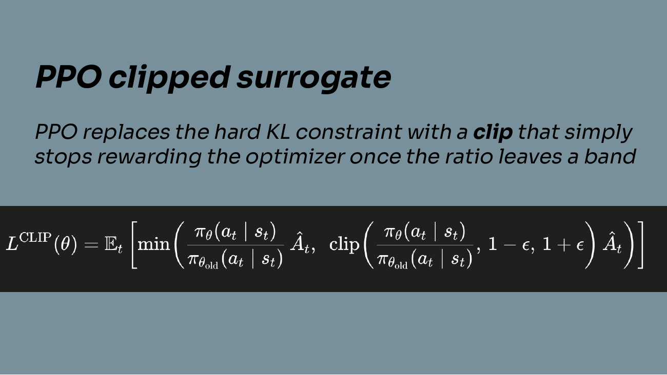
The slide’s phrase about leaving a band is shorthand. With a positive advantage, only an increase beyond the upper bound loses further objective benefit. With a negative advantage, only a decrease below the lower bound does so. Movement in the harmful direction still affects the objective, and clipping never forcibly returns the model probability to the band. The worked positive and negative cases in Section 3.5 make this distinction explicit.¹⁷

---

1. Yu, Q., et al. (2025). DAPO: An open-source LLM reinforcement learning system at scale. Advances in Neural Information Processing Systems, 38. DOI: 10.52202/085713-3775. Source. Link checked 2026-09-16. Sections 3.1–3.4. These are separate controls, not a guarantee of correct reasoning.

2. Rafailov, R., Sharma, A., Mitchell, E., Manning, C. D., Ermon, S., & Finn, C. (2023). Direct Preference Optimization: Your language model is secretly a reward model. Advances in Neural Information Processing Systems, 36. Source. Link checked 2026-09-16. DPO objective. Standard offline objective with a fixed reference.

3. Schulman, J., Moritz, P., Levine, S., Jordan, M. I., & Abbeel, P. (2016). High-dimensional continuous control using generalized advantage estimation. International Conference on Learning Representations. Source. Link checked 2026-09-16. Advantage-estimation equations. Bias and variance depend on discount, trace parameter and value estimates.

4. Shao, Z., et al. (2024). DeepSeekMath: Pushing the Limits of Mathematical Reasoning in Open Language Models (arXiv:2402.03300). Source. Link checked 2026-09-16. Section 4. Removing the learned critic does not remove grouped-rollout storage.

5. Hu, E. J., et al. (2022). LoRA: Low-rank adaptation of large language models. International Conference on Learning Representations. arXiv. Link checked 2026-09-16. Section 4.1, equation 3. Savings in trainable parameter count are not equal savings in total memory or runtime. The 4096-by-4096 rank16 count below is worked arithmetic using illustrative dimensions, not a benchmark result.

6. Schulman, J., Wolski, F., Dhariwal, P., Radford, A., & Klimov, O. (2017). Proximal Policy Optimization Algorithms. arXiv:1707.06347. Source. Link checked 2026-09-16. Section 3, equation 7. Section 3, equation 7 and Figure 1. The bound applies to a surrogate term, not directly to the resulting policy. The numerical examples illustrate the formula, not measured training behavior.

7. Ouyang, L., et al. (2022). Training language models to follow instructions with human feedback. Advances in Neural Information Processing Systems, 35, 27730–27744. DOI: 10.52202/068431-2011. Official proceedings. Link checked 2026-09-16. Methods. Supervised fine-tuning stage. This describes the classical reward-model recipe, not every method using human feedback. Examples and task distribution determine the supported behavior.

8. Lambert, N., Morrison, J., Pyatkin, V., et al. (2024). Tülu 3: Pushing Frontiers in Open Language Model Post-Training (arXiv:2411.15124, v5). Source. Link checked 2026-09-16. RLVR stage. A verifier checks only the conditions encoded by its tests.

9. Ouyang, L., et al. (2022). Training language models to follow instructions with human feedback. Advances in Neural Information Processing Systems, 35, 27730–27744. DOI: 10.52202/068431-2011. Official proceedings. Link checked 2026-09-16. Methods. Supervised fine-tuning stage. This describes the classical reward-model recipe, not every method using human feedback. Examples and task distribution determine the supported behavior.

10. Hugging Face. (2025). TRL: Transformer Reinforcement Learning (v0.22.2 documentation). Official documentation. Link checked 2026-09-16. Version 0.22.2. Official API documentation. Installed versions can differ.

11. Wolf, T., et al. (2020). Transformers: State-of-the-art natural language processing. Proceedings of the 2020 Conference on Empirical Methods in Natural Language Processing: System Demonstrations (pp. 38–45). Association for Computational Linguistics. DOI: 10.18653/v1/2020.emnlp-demos.6. Paper. Link checked 2026-09-16. Section 3, Figure 2. Tokenizer and model head must match the checkpoint.

12. Paszke, A., et al. (2019). PyTorch: An imperative style, high-performance deep learning library. Advances in Neural Information Processing Systems, 32. Original paper. Link checked 2026-09-16. Sections 2 and 5.1. Section 4.3. This describes the library’s numerical representation. The user must still supply the intended differentiable objective.

13. Lhoest, Q., et al. (2021). Datasets: A community library for natural language processing. Proceedings of the 2021 Conference on Empirical Methods in Natural Language Processing: System Demonstrations (pp. 175–184). Association for Computational Linguistics. DOI: 10.18653/v1/2021.emnlp-demo.21. Paper. Link checked 2026-09-16. Section 3, S1–S4. Splitting functions do not by themselves prove absence of leakage.

14. Paszke, A., et al. (2019). PyTorch: An imperative style, high-performance deep learning library. Advances in Neural Information Processing Systems, 32. Original paper. Link checked 2026-09-16. Sections 2 and 5.1. Section 4.3. This describes the library’s numerical representation. The user must still supply the intended differentiable objective.

15. Hugging Face. (2025). Accelerate (Accelerate v1.10.1 documentation). Official documentation. Link checked 2026-09-16. Version 1.10.1, Accelerator and prepare. Versioned API guidance, not a throughput guarantee.

16. Hu, E. J., et al. (2022). LoRA: Low-rank adaptation of large language models. International Conference on Learning Representations. arXiv. Link checked 2026-09-16. Section 4.1, equation 3. Savings in trainable parameter count are not equal savings in total memory or runtime. The 4096-by-4096 rank16 count below is worked arithmetic using illustrative dimensions, not a benchmark result.

17. Schulman, J., Wolski, F., Dhariwal, P., Radford, A., & Klimov, O. (2017). Proximal Policy Optimization Algorithms. arXiv:1707.06347. Source. Link checked 2026-09-16. Section 3, equation 7. Section 3, equation 7 and Figure 1. The bound applies to a surrogate term, not directly to the resulting policy. The numerical examples illustrate the formula, not measured training behavior.