4  Evaluation-based system improvement

Chapters 1 through 3 produced a versioned model request and a record of which context the application selected. One convincing answer still cannot show that a change helps across different user groups and case types, repeated trials, or required latency and cost limits. Evaluation-driven development (EDD) is the book’s engineering workflow for treating every proposed improvement as an experiment with fixed test inputs, defined scoring rules, an estimate of uncertainty, and a release decision. The NIST AI Risk Management Framework¹ likewise places measurement inside lifecycle risk management. The name and exact EDD loop are the book’s synthesis, not an external standard. The front matter maps each step to the NIST framework and related ISO/IEC standards.

Figure 4.1: Evaluation-driven development starts from product requirements, fixes the cases, compares one change with a baseline, records each run, and turns uncertainty and slice results into a release decision.

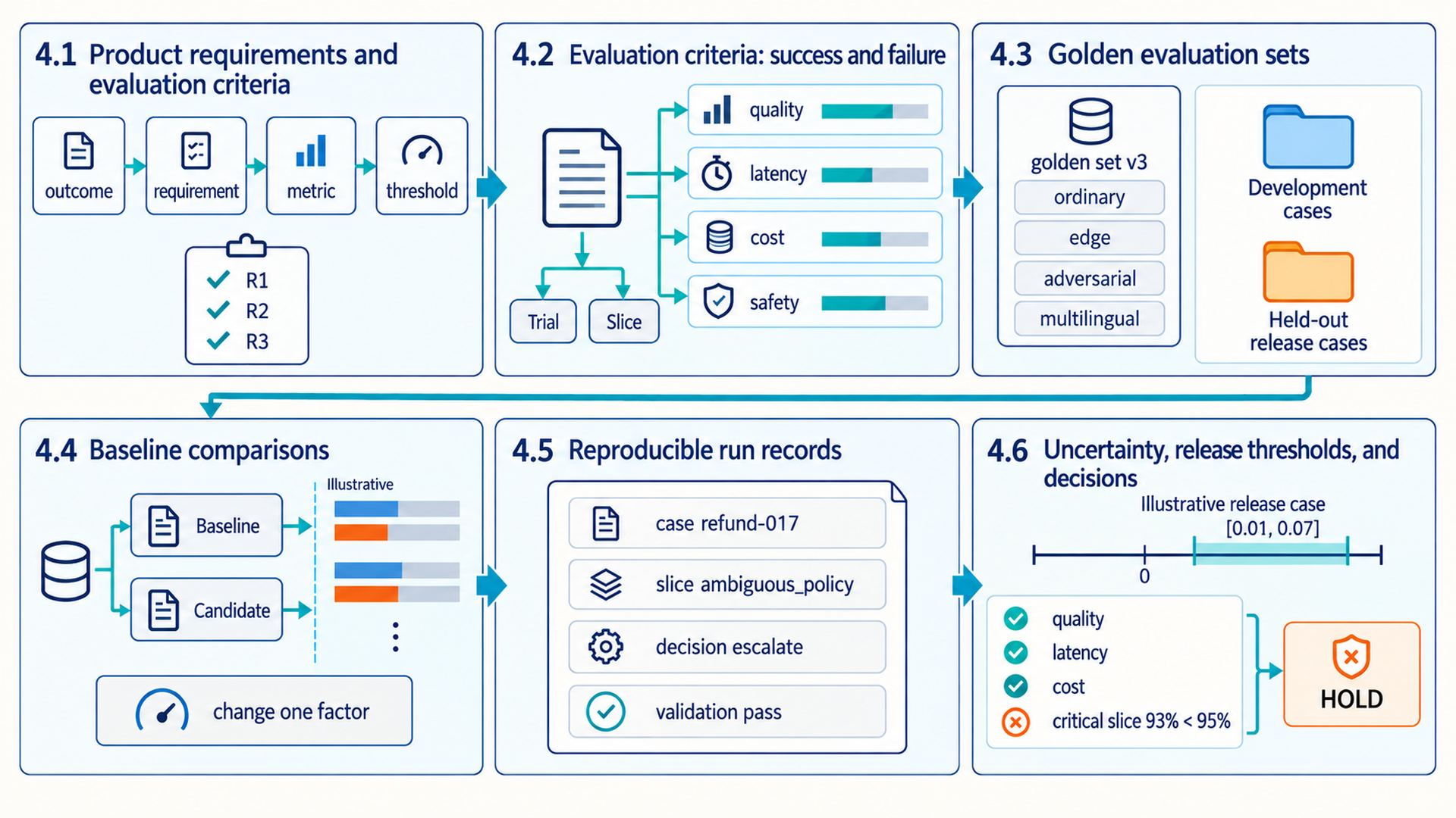
The map connects product requirements to test cases, comparisons with the current system, run records, and checks that decide whether a change can be released. An isolated score needs a description of the cases tested and the costs of failure before it can support a decision. The final panel illustrates the release case in Section 4.6: the quality interval is positive, but a required slice is below its threshold, so the candidate is held.

4.1 Product requirements and evaluation criteria

Chapter 2 defined a task specification for one request. A product needs requirements before that: what it must achieve for its users and organization, and what it must never do. A product requirement is a verifiable statement of required or forbidden system behavior under stated conditions, traced to a product outcome. “Escalate every ticket that needs a person” is a requirement. “Use the largest available model” is a design choice.

Requirements come from the business value the product must deliver, its users and their tolerance for delay or error, domain experts, legal and policy obligations, and the process the product replaces. The NIST AI Risk Management Framework asks organizations to document business value, risk tolerance, and system requirements elicited from the relevant people (MAP 1.4 to 1.6). It also asks them to examine the costs of expected errors (MAP 3.2).² ISO/IEC/IEEE 29148 specifies requirements-engineering processes and records for systems and software in general.³

A requirement becomes testable through a chain: product outcome, requirement, measurement, threshold, and the evaluation cases that exercise it. The measurement is usually a proxy metric, an offline measurement used in place of a product outcome observable only in production. Recall on labeled escalations is the fraction of tickets requiring escalation that the system correctly escalates. It measures whether those customers are routed to a person. Measuring the delay requires a separate timing check. Section 13.4 describes how production data tests whether a proxy predicts the outcome.

Table 4.1: Each requirement links a product outcome to a measurement and a threshold source.

Product outcome	Requirement	Measurement	Threshold source
Urgent customers get a person without delay	Escalate every ticket that needs a person	Recall on the escalation slice	Current manual triage
Triage costs less than manual handling	Stay within the cost per ticket	Model cost plus human-review cost per ticket	Product budget
Customer data stays private	Never show one customer another customer’s data	Cross-customer disclosures in adversarial cases (veto)	Legal and policy obligation
Customers get answers while they wait	Answer within the latency limit	p95 latency on representative traffic	Measured user tolerance

A threshold value needs a source that exists before any candidate is scored: the performance of the current process, the product budget, a legal obligation, or a measured user tolerance.

Example: Thresholds from the current process and the budget

This example uses a different requirement from escalating every eligible ticket: the system must miss no more required escalations than staff do. An audit of 200 manually triaged tickets finds 40 required escalations. Staff missed 2 of them, a recall of 38 / 40 = 0.95, and manual triage costs $3.00 per ticket.

1. The system may miss no more escalations than staff do, so the recall floor on the escalation slice is 0.95. 2. The product goal halves the triage cost to $1.50 per ticket. A model call costs $0.02, and each ticket sent to human review costs $3.00. 3. With review rate \(r\), the cost per ticket is \(0.02 + 3.00r \le 1.50\), so \(r \le 1.48 / 3\), about \(0.4933\). Result: The release gate requires escalation recall of at least 0.95 and sends at most 49 percent of tickets to human review, rounding the cost-derived ceiling down conservatively.

Interpretation: With 40 escalations, an observed recall of 0.95 has a 95 percent Wilson interval from about 0.83 to 0.99 (Section 9.7). The escalation slice needs more cases before this floor can separate a candidate from a weaker one.

Requirements for open-ended outputs often change after people read real outputs. Shankar and colleagues call this criteria drift: people need criteria to grade outputs, and grading outputs helps them define the criteria.⁴ The requirement list is versioned with the golden set, and a changed requirement starts a new evaluation version (Section 4.3).

A completeness check finds qualities that still lack a requirement. ISO/IEC 25059 defines quality characteristics for AI systems and describes them as a set against which stated quality requirements can be compared for completeness.⁵

Requirement traceability links each requirement to its measurement, threshold, evaluation cases, and results. With stable requirement identifiers, a release decision record can list each requirement with its result: passed, failed, or not tested. Section 13.3 shows how evaluation results and blocking failures support PASS or HOLD. A veto requirement is mandatory: its failure blocks release, producing HOLD. Section 4.2 turns the requirements into an evaluation specification.

4.2 Evaluation criteria: success and failure

A deterministic program often has one expected output for one input. Language tasks often have several valid outputs, raters frequently disagree, and an improvement in one quality can reduce another. The evaluation specification restates the requirements from Section 4.1 as measurable qualities and failure costs.

An answer can be factually correct but too slow, unsafe, unsupported, or expensive. It can satisfy an automated text metric while violating the user’s intent. Model versions and benchmarks also change quickly, so a public benchmark score cannot replace product-specific evaluation criteria.

In Chapter 1, evaluation meant running held-out cases and recording measurements without updating the model. As a product procedure, an evaluation runs a versioned system on specified cases, scores observable outcomes, and supplies evidence for a decision. Two more terms identify each attempt and the subsets compared across cases:

• Trial: One attempt at one evaluation task. Because sampling, retrieval, and tools can vary, the same system can produce different answers across trials.

• Slice: A defined subset of evaluation cases, such as language, customer tier, risk level, query type, document length, or tool requirement.

The evaluation specification then records four groups of measurements:

• Quality: correctness, relevance, groundedness (support for claims in the supplied evidence), completeness, style, or task success.
• Operational behavior: latency (time to complete a request), throughput (requests completed per unit of time), failure rate, token use, and monetary cost.
• Safety and policy: refusal behavior, harmful content, authorization, privacy, and escalation.
• Reliability: variation in scores across trials, environments, model versions, and data slices. Variance is a statistical measure of that spread.

Each dimension has its own measurement method and decision rule.

Aggregation can summarize ordinary variation, while veto conditions protect non-negotiable behavior. A high average cannot compensate for exposing private data or executing an unauthorized action. The evaluation record keeps per-example scores and slice labels alongside any headline metric, allowing a release decision to distinguish broad improvement from a severe local regression.

4.3 Golden evaluation sets

Evaluation criteria state which product outcomes matter, but they do not supply the cases used to measure them. A convenient sample can overrepresent easy cases and hide failures that would cause the most harm. The evaluation therefore needs a versioned collection of representative and risk-focused cases.

A golden set is that versioned collection of evaluation tasks, each with an expected outcome or grading criterion. It can combine human-authored cases, de-identified production samples, synthetic variations, and adversarial tests. CheckList⁶ supports organizing focused behavioral tests by capability and test type, but the exact mixture and maintenance policy here are product decisions. Production records should be de-identified or handled under the product’s privacy controls.

Evaluation cases should start from product decisions. A support-routing system needs ordinary FAQ cases, legitimate escalations, ambiguous cases, out-of-scope requests, multilingual messages, and policy-conflict cases. If missing an escalation is costly, the evaluation should report that slice separately and can oversample it to include more cases. After oversampling, an overall score reflects production traffic only if slice results are reweighted to their traffic shares.

Synthetic evaluation data

Synthetic cases cover known dimensions and failure hypotheses that are underrepresented in available production data. They are useful when new features lack production volume, rare safety edge cases require testing, or a test must isolate one changed condition.

Start from a written specification, generate candidate cases, remove duplicates, and have people or deterministic rules validate the labels. Synthetic cases expand coverage, while real failures keep the suite connected to actual product behavior.

Limitation: A generator reproduces its own assumptions and may miss real user language or operational constraints.

Hidden stratification

An overall score can rise while a critical subgroup declines. Important slice results should appear beside the headline metric, with enough examples to diagnose why the slice moved.

A baseline comparison is valid only when it changes the intended variable and preserves the remaining conditions. Section 4.5 lists the conditions a run record keeps.

Repeated runs are relevant when sampling, routing, tools, or environment state introduce variation. The comparison reports the distribution of outcomes across the full run set. Development cases guide tuning, while held-out release cases test the resulting system. Repeatedly tuning against the release cases can fit their particular answers and weaken the evidence about unseen requests. The golden set is also maintained: traffic, requirements, observed failures, and risks can require new cases or renewed label review. When data, rubric, or judge changes are necessary, the protocol record marks a new version so the result is not presented as a direct continuation of an older score.

4.4 Baseline comparisons

The golden set now keeps representative cases and risk-focused slices visible across versions. A comparison cannot support a reliable conclusion when the model, prompt, retrieval, workflow, or scoring setup changes without a recorded baseline. In EDD, the golden set is run against the versioned baseline and a system with one controlled factor changed. Both runs use the same scoring procedure and otherwise fixed settings in comparable environments. Under those conditions, the measured difference estimates the effect of the change rather than a mixture of unrelated changes.

EDD adapts test-driven development, in which tests are written before the code they check, to systems with probabilistic outputs and imperfect proxies. An evaluation run (eval) combines fixed cases, a scoring procedure, a comparison target, and the product decision it informs. The eval specification is versioned because user behavior and models change.

1. Define the behavior and observable final state the product must achieve.
2. Create and version representative cases and risk-focused slices before tuning.
3. Run the current system on the fixed set and store outputs, traces, latency, cost, and version metadata.
4. Change one model, prompt, retrieval, workflow, or policy factor. Use this as the default comparison method. When two factors may interact, run a planned multi-factor experiment rather than assuming the one-factor result will generalize.
5. Rerun the same evaluation, estimate uncertainty, and inspect failures.
6. Release, revise, or revert according to the decision rule, and add new failures to the suite.

Defining the eval before inspecting a preferred output helps it measure the underlying behavior across cases.

A score without the input set, system version, trace, and decision threshold cannot be reproduced or interpreted safely.

The fixed set keeps ordinary, boundary, adversarial, and production-derived cases visible in the comparison. Validated production failures can become regression cases after privacy review and label validation. Duplicate or near-duplicate cases must be controlled across development and held-out partitions, and each case record must retain its expected outcome, rubric version, source record, and label review status.

4.5 Reproducible run records

Reproducing a comparison requires a record of the system and conditions that produced every case result. A run configuration records the case-set revision, model, prompt, context policy, retrieval index, tools, decoder settings, random seed, judge versions, and runtime environment. Each result row stores that configuration beside one case’s raw output, parsed output, validation result, trace, latency, token use, tool calls, citations, and evidence of the system’s final outcome. Together these records make the baseline reproducible and reviewable. Pineau and colleagues⁷ recommend preserving code, data, checklists, and experimental conditions. The field list here is the book’s design.

In the shortened harness below, case supplies the ID, slice, and input. config is a dataclass instance containing the fixed run settings. system accepts the input and configuration and returns an object with the output, validation, trace, and usage fields accessed in the code. The harness times the call and combines those values into one row. It does not define the system under test, and it records only calls that return those fields successfully. The calling runner must separately record exceptions and timeouts as failed trials rather than omit them from the results.

Code example: An evaluation harness keeps configuration and per-case evidence together.

from dataclasses import asdict
from time import perf_counter

def run_case(case, system, config):
    started = perf_counter()
    response = system(case.input, config=config)
    elapsed_ms = 1000 * (perf_counter() - started)
    return {
        "case_id": case.id,
        "slice": case.slice,
        "config": asdict(config),
        "raw_output": response.raw_output,
        "parsed_output": response.parsed_output,
        "validation": response.validation,
        "trace": {
            "tool_calls": response.trace.tool_calls,
            "citations": response.trace.citations,
            "final_state_evidence": response.trace.final_state_evidence,
        },
        "input_tokens": response.usage.input_tokens,
        "output_tokens": response.usage.output_tokens,
        "latency_ms": elapsed_ms,
    }

Example: One harness call produces one reviewable row

Case refund-017 belongs to the ambiguous_policy slice and contains a question about whether an opened item is returnable. Configuration prompt-v3/model-a/temp-0 is passed unchanged to the system. The returned row keeps that configuration beside the raw answer, parsed decision escalate, validation result pass, input and output token counts, and measured latency. A later metric calculation can use the parsed decision, while an error review can still inspect the original answer and trace.

The harness only preserves observations. Metrics and release thresholds are calculated from them later. When retrieval or model sampling can vary, the same case is run several times and each trial remains a separate record.

4.6 Uncertainty, release thresholds, and decisions

A controlled dataset makes runs of the baseline and changed system comparable. However, test sets are limited, and models generate text unpredictably. A small score improvement might just be random noise. A quality gain can also violate latency, cost, or safety limits.

Three checks answer those risks in turn: a bootstrap interval estimates sampling uncertainty in the observed difference, slice analysis exposes a change that improves the average while breaking a specific case type, and a release gate tests latency, cost, and safety limits alongside quality.

A bootstrap confidence interval estimates sampling uncertainty by drawing from the observed evaluation cases with replacement and recomputing the statistic. Each resample contains as many cases as the original set. “With replacement” means a case can appear more than once while another is absent. For a paired comparison, each selected case carries both its baseline and candidate scores, so the comparison keeps the same case difficulty on both sides. Repeating this process gives a distribution of resampled statistics. Its selected percentiles form the interval. A nominal 95 percent confidence interval aims to cover the population value in 95 percent of repeated evaluations under the method’s sampling assumptions. It is not a 95 percent probability that this particular candidate improves the product. Efron⁸ established the bootstrap method. Bouthillier and colleagues⁹ show that data sampling, initialization, and hyperparameter choices can all affect benchmark comparisons, so one percentile interval over cases does not capture every source of variation.

\[ CI_{1-\alpha}=[q_{\alpha/2}(m_{1:B}),q_{1-\alpha/2}(m_{1:B})] \tag{4.1}\]

Here, \(m_b\) is the metric or paired metric difference calculated on bootstrap sample \(b\), \(B\) is the number of resamples, \(q\) selects empirical quantiles, and \(\alpha\) is the nominal error rate. This is the intended rate rather than a guaranteed rate for this sample. A quantile identifies a position in the sorted resampled statistics, with interpolation between values when the selected convention requires it. For a 95 percent interval, set \(\alpha=0.05\): the lower endpoint is the 0.025 quantile, near the bottom 2.5 percent, and the upper endpoint is the 0.975 quantile, near the top 2.5 percent. The interval estimates variation from sampling cases using the observed set. It does not correct label bias, benchmark contamination, user correlation, production distribution shift, or a metric that fails to represent the product decision. Repeated model or tool trials address run-to-run variation separately.

Example: Paired bootstrap interval

Four cases have baseline scores \((0.60, 0.80, 0.50, 0.90)\) and treatment scores \((0.70, 0.75, 0.55, 0.95)\). Pair each treatment score with its own baseline score before resampling, giving deltas \((+0.10, -0.05, +0.05, +0.05)\). The observed mean improvement is \(0.0375\).

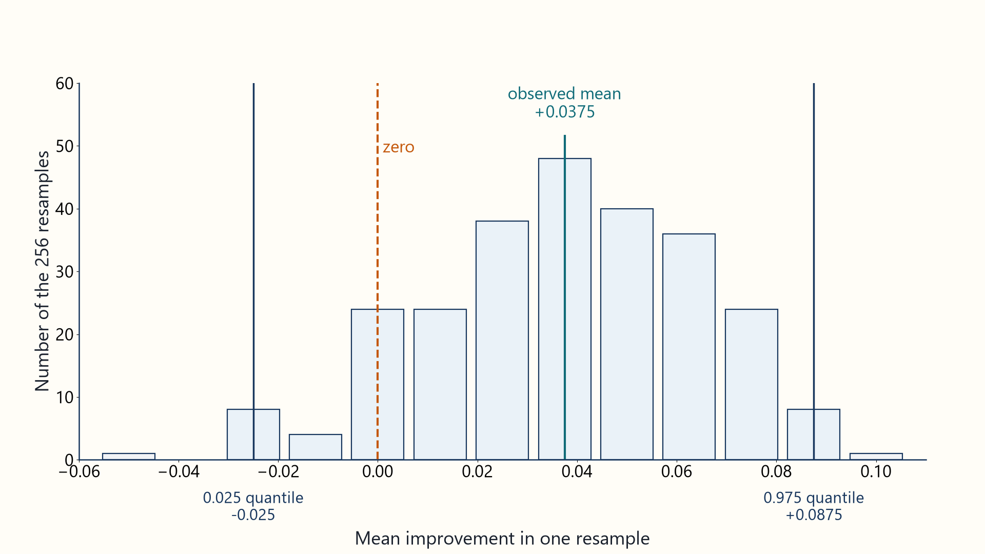
1. A resample can select cases 1, 1, 3, and 4, producing deltas \((+0.10, +0.10, +0.05, +0.05)\) and a mean of \(+0.075\). 2. Another can select cases 2, 2, 3, and 4, producing \((-0.05, -0.05, +0.05, +0.05)\) and a mean of \(0\). 3. For this four-case illustration, enumerate all \(4^4 = 256\) ordered resamples. Using linear interpolation between sorted values for empirical quantiles, the 0.025 and 0.975 quantiles are \(-0.025\) and \(0.0875\). Result: The interval is \([-0.025, 0.0875]\). It includes zero, so this small case set does not establish a positive improvement.

Interpretation: Pairing keeps each case’s baseline and treatment together. A larger evaluation set still needs a stated resample count, seed, and quantile convention.

The figure counts the means of all 256 resamples. The nominal 95 percent percentile interval runs from -0.025 to 0.0875, so zero stays inside the interval. With this discrete distribution, the fraction of resample means between the endpoints need not be exactly 95 percent.

Figure 4.2: All 256 bootstrap resamples of the four-case example give an interval from -0.025 to 0.0875, which includes zero.

NumPy, imported as np, is a library for numerical arrays. The function below accepts two non-empty one-dimensional sequences of finite scores in matching case order. It computes per-case differences and returns two endpoints for their mean difference. Each draw selects as many case positions as the original set and keeps both systems’ scores paired. draws must be a positive integer. A fixed seed makes these draws repeatable in the recorded runtime, and method="linear" specifies the empirical quantile convention.

Code example: Paired resampling estimates a percentile interval for the mean per-case score difference.

import numpy as np

def paired_bootstrap_delta_ci(baseline, treatment, draws=10_000, seed=17):
    baseline = np.asarray(baseline, dtype=float)
    treatment = np.asarray(treatment, dtype=float)
    if (baseline.ndim != 1 or treatment.ndim != 1
            or baseline.shape != treatment.shape or baseline.size == 0):
        raise ValueError("scores need matching non-empty one-dimensional arrays")
    if not (np.isfinite(baseline).all() and np.isfinite(treatment).all()):
        raise ValueError("scores must be finite")
    if isinstance(draws, (bool, np.bool_)) or not isinstance(draws, (int, np.integer)) or draws <= 0:
        raise ValueError("draws must be a positive integer")
    with np.errstate(over="ignore", invalid="ignore"):
        deltas = treatment - baseline
    if not np.isfinite(deltas).all():
        raise ValueError("score differences must be finite")
    rng = np.random.default_rng(seed)
    try:
        with np.errstate(over="raise", invalid="raise"):
            estimates = [
                deltas[rng.integers(0, len(deltas), size=len(deltas))].mean()
                for _ in range(draws)
            ]
            if not np.isfinite(estimates).all():
                raise ValueError("scores exceed the supported numeric range")
            endpoints = np.quantile(estimates, [0.025, 0.975], method="linear")
            if not np.isfinite(endpoints).all():
                raise ValueError("scores exceed the supported numeric range")
    except FloatingPointError as error:
        raise ValueError("scores exceed the supported numeric range") from error
    return tuple(endpoints)

Calling the function with the four-case scores above gives a random-sampling estimate of the enumerated interval. For these four cases, there are only 12 distinct resample means. With the default 10,000 draws and seed 17, the estimated endpoints match the enumerated interval in the recorded runtime. With fewer draws, such as 200, the endpoints can differ across seeds. A larger case set can have many more distinct resample means, so sampled endpoints can also vary with seed or draw count. Input shape, finiteness and draw-count checks run before resampling. Numeric overflow during resampling or interval calculation also raises ValueError.

Other methods compare systems under different assumptions. A paired t-test tests the mean of independent per-case differences. Its usual exact test assumes normally distributed differences. With many independent cases and finite variance, the mean may be approximately normal even when individual differences are not. McNemar’s test compares paired pass/fail outcomes by counting cases on which only one system passes. Bootstrap resampling can estimate uncertainty for medians, ratios, or rank metrics without a formula for their sampling distributions, but each resample must recompute the chosen statistic. The function above implements only a mean paired difference. Dror and colleagues¹⁰ compare tests for language-processing experiments, and Miller¹¹ discusses paired comparisons and clustered errors when several cases share a source. Under an unchanged independent sampling design, interval width for a mean often shrinks roughly with the square root of the number of cases: quadrupling the case set about halves the width. Correlated cases or a different case mixture can invalidate that estimate.

The resampling unit must match the independence assumption. When one user contributes many correlated requests, a cluster bootstrap draws users and keeps each selected user’s request group together. Sessions can serve the same purpose when they are the independent groups. The statistic must still match the product question: averaging equally over users and averaging equally over requests measure different quantities. The case-level function above does not implement this grouped resampling. A release gate can require minimum quality gains and prevent critical-slice regressions, while capping p95 latency, task cost, and policy violations. Here p95 latency is the 0.95 quantile of measured request completion times, with the empirical quantile convention recorded for finite samples.

Example: A release gate combines requirements

Consider a candidate with a quality interval of \([0.01, 0.07]\), critical-slice success of 93%, p95 latency of 760 ms, and cost of $0.018 per task. The release rule requires a positive lower interval endpoint, at least 95% critical-slice success, p95 latency no greater than 800 ms, and cost no greater than $0.020.

1. The interval, latency, and cost pass their stated requirements. 2. The critical slice fails: 93% is below 95%. Result: Hold the candidate. An average quality improvement does not cancel a failed critical slice.

These values are illustrative. A production gate must state its mandatory checks before examining the candidate results.

A release decision needs both an estimated change and defined limits for every critical slice, cost, latency, and policy condition. Chapter 5 examines how automatic metrics, judge models, human ratings, and benchmarks supply those measurements and where each can mislead.

---

1. Tabassi, E. (2023). Artificial Intelligence Risk Management Framework (AI RMF 1.0) (NIST AI 100-1). National Institute of Standards and Technology. https://doi.org/10.6028/NIST.AI.100-1. The framework supports lifecycle risk governance and measurement. It does not define the book’s EDD workflow.

2. Tabassi, E. (2023). Artificial Intelligence Risk Management Framework (AI RMF 1.0) (NIST AI 100-1). National Institute of Standards and Technology. https://doi.org/10.6028/NIST.AI.100-1. MAP 1.4 to 1.6 cover business value, risk tolerance, and elicited system requirements, and MAP 3.2 covers the costs of expected errors. The framework is voluntary and does not prescribe metrics or thresholds.

3. International Organization for Standardization, International Electrotechnical Commission, & Institute of Electrical and Electronics Engineers. (2018). Systems and software engineering: Life cycle processes: Requirements engineering (ISO/IEC/IEEE 29148:2018). https://www.iso.org/standard/72089.html. The standard specifies requirements-engineering processes and the information items they produce. It is not specific to AI systems.

4. Shankar, S., Zamfirescu-Pereira, J. D., Hartmann, B., Parameswaran, A. G., & Arawjo, I. (2024). Who validates the validators? Aligning LLM-assisted evaluation of LLM outputs with human preferences. In Proceedings of the 37^th Annual ACM Symposium on User Interface Software and Technology (pp. 1–14). Association for Computing Machinery. https://doi.org/10.1145/3654777.3676450. The observation comes from a qualitative study of an evaluation-assistant tool.

5. International Organization for Standardization & International Electrotechnical Commission. (2023). Software engineering: Systems and software Quality Requirements and Evaluation (SQuaRE): Quality model for AI systems (ISO/IEC 25059:2023). https://www.iso.org/standard/80655.html. The standard extends the SQuaRE quality model for AI systems. It defines quality characteristics, not threshold values.

6. Ribeiro, M. T., Wu, T., Guestrin, C., & Singh, S. (2020). Beyond accuracy: Behavioral testing of NLP models with CheckList. In Proceedings of the 58^th Annual Meeting of the Association for Computational Linguistics (pp. 4902–4912). Association for Computational Linguistics. https://doi.org/10.18653/v1/2020.acl-main.442. CheckList supports capability-focused cases, not a universal golden-set composition.

7. Pineau, J., Vincent-Lamarre, P., Sinha, K., Larivière, V., Beygelzimer, A., d’Alché-Buc, F., Fox, E., & Larochelle, H. (2021). Improving reproducibility in machine learning research: A report from the NeurIPS 2019 reproducibility program. Journal of Machine Learning Research, 22(164), 1–20. https://jmlr.org/papers/v22/20-303.html.

8. Efron, B. (1979). Bootstrap methods: Another look at the jackknife. The Annals of Statistics, 7(1), 1–26. https://doi.org/10.1214/aos/1176344552. The source establishes the resampling method. The interval type and resampling unit still require an evaluation-specific choice.

9. Bouthillier, X., Delaunay, P., Bronzi, M., Trofimov, A., Nichyporuk, B., Szeto, J., Sepah, N., Raff, E., Madan, K., Voleti, V., Kahou, S. E., Michalski, V., Serdyuk, D., Arbel, T., Pal, C., Varoquaux, G., & Vincent, P. (2021). Accounting for variance in machine learning benchmarks. arXiv. https://arxiv.org/abs/2103.03098. The paper supports accounting for several sources of variation, not treating one bootstrap interval as complete uncertainty analysis.

10. Dror, R., Baumer, G., Shlomov, S., & Reichart, R. (2018). The hitchhiker’s guide to testing statistical significance in natural language processing. In Proceedings of the 56^th Annual Meeting of the Association for Computational Linguistics, Volume 1: Long Papers (pp. 1383–1392). Association for Computational Linguistics. https://doi.org/10.18653/v1/P18-1128. The paper surveys significance tests and their assumptions for NLP comparisons. It does not choose a test for a particular product metric.

11. Miller, E. (2024). Adding error bars to evals: A statistical approach to language model evaluations. arXiv. https://arxiv.org/abs/2411.00640. The paper gives standard errors, paired comparisons, clustered errors, and sample-size planning for language-model evaluations. Its formulas assume the stated sampling model.